Luenberger Observers for State Estimation

The Problem: Unmeasurable States

First, let's get a clear picture of the problem we're solving. The controllers we've designed require the full state vector $x$ at every instant in time. What happens when we can't measure it?

A First Attempt: The Open-Loop Observer

A natural first thought might be to build a software model of our system. Since we know the system matrices ($A,B,C$) and the control input $u$ we are sending, we could run a simulation in parallel with the real system and use the simulation's state as our estimate.

This is called an open-loop observer or a real-time simulator. Its dynamics would simply be:
$\dot{\hat{x}}=A\hat{x}+Bu$
Here, $\hat{x}$ (read "x-hat") represents our estimate of the true state $x$.

While simple, this approach has significant flaws.

As the video highlights, the open-loop observer is "stupid" because it ignores a valuable piece of information we have access to: the actual measured output of the plant, $y$.

The Solution: The Luenberger Observer

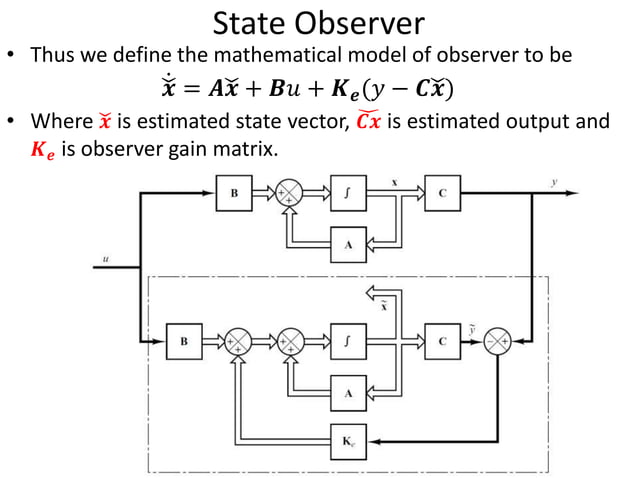
The key innovation of the Luenberger observer is to use the discrepancy between the plant's actual output ($y$) and the observer's estimated output ($\hat{y}$) to continuously correct the state estimate. This creates a closed-loop observer.

The structure is as follows:

1. The observer generates an estimated output: $\hat{y}=C\hat{x}$.
2. It compares this to the measured output from the plant, $y$, to form an output error: $y-\hat{y}$.
3. This error is multiplied by an observer gain matrix, $L$, and fed back as a correction term into the observer's dynamics.

The governing equation for the Luenberger observer is:
$\dot{\hat{x}}=A\hat{x}+Bu+L(y-\hat{y})$
Substituting $\hat{y}=C\hat{x}$, we get:
$\dot{\hat{x}}=A\hat{x}+Bu+L(y-C\hat{x})$

The term $L(y-C\hat{x})$ is the correction mechanism. If the estimated output matches the real output, this term is zero. If they differ, this term nudges the dynamics of $\hat{x}$ to reduce the error. The observer gain $L$ determines how strongly the observer reacts to this output error.

The block diagram below provides a great visual representation of this structure.

The Core Principle: Error Dynamics

This structure is intuitive, but does it actually work? We need to prove that our state estimate $\hat{x}$ will converge to the true state $x$. To do this, we analyze the dynamics of the estimation error, which we define as $e=x-\hat{x}$. Our goal is to show that $e(t)\to 0$.

The rate of change of the error is $\dot{e}=\dot{x}-\dot{\hat{x}}$. Let's substitute the equations for the plant and the observer:
$\dot{x}=Ax+Bu$
$\dot{\hat{x}}=A\hat{x}+Bu+L(y-C\hat{x})$
Assuming an ideal plant with no disturbances and $y=Cx$:
$\dot{e}=(Ax+Bu)-(A\hat{x}+Bu+L(Cx-C\hat{x}))$
The $Bu$ terms cancel out:
$\dot{e}=Ax-A\hat{x}-L(Cx-C\hat{x})$
Factoring out the state terms and the error $e$:
$\dot{e}=A(x-\hat{x})-LC(x-\hat{x})$
$\dot{e}=(A-LC)e$

This is the fundamental result for the Luenberger observer. The estimation error has its own dynamics, completely independent of the control input $u$. For the error $e$ to decay to zero from any initial condition, this linear system must be stable. This means all eigenvalues of the matrix $(A-LC)$ must be in the left half of the complex plane.

This brings us to the crucial link with a concept from Module 2: observability. It turns out that we can place the eigenvalues of $(A-LC)$ anywhere we want by choosing the observer gain $L$ if and only if the system pair $(A,C)$ is observable. This makes perfect sense: if a state is unobservable, it has no effect on the output $y$, so the output error $y-\hat{y}$ contains no information about that state's error, and the observer can't correct it.

Let's watch the final segment of the video to see this derivation and conclusion in action.

Conclusion

In this lesson, we have established the fundamental principle of the Luenberger observer as a tool for estimating unmeasured system states.

Key Takeaways:

• State feedback controllers require full state information, which is often unavailable in practice.
• A simple open-loop simulation of the system is not a robust estimator because it cannot correct for errors and fails if the system is unstable.
• The Luenberger observer is a closed-loop estimator that uses the output error ($y-\hat{y}$) as a correction term.
• The observer's governing equation is $\dot{\hat{x}}=A\hat{x}+Bu+L(y-C\hat{x})$, where $L$ is the observer gain matrix.
• The estimation error dynamics are given by $\dot{e}=(A-LC)e$.
• For the state estimate to converge to the true state, the error dynamics must be stable. This is achieved by choosing $L$ such that all eigenvalues of $(A-LC)$ are stable.
• The ability to arbitrarily place these error-dynamics poles depends on the system's observability.

Preview of the Next Lesson:
We've learned why the observer works and that we need to choose the gain matrix $L$ to make $(A-LC)$ stable. But how should we choose $L$? What are "good" locations for the observer's poles? In the next lesson, we will answer these questions by learning how to select observer pole locations to achieve a desired estimation speed and then calculate the observer gain matrix $L$ to place them there.