MIMO Decoupling with Static State Feedback

The Goal: A Diagonal System

Ideally, we would want our system to be naturally decoupled. For a 2-input, 2-output system, this would look like the diagram below, where the controller K(s) is diagonal.

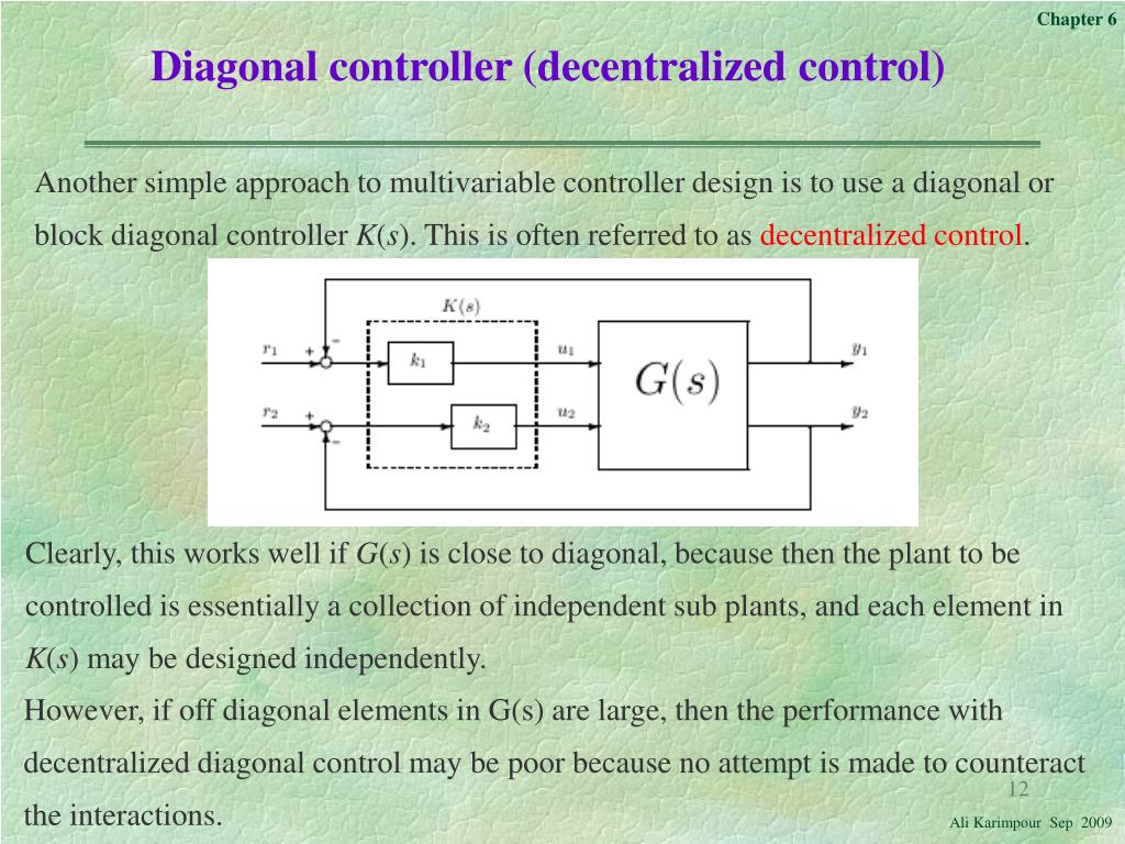
As the diagram explains, this simple "decentralized" approach works well only if the plant G(s) is already "nearly diagonal"—meaning the interactions between channels are weak. But what if they are strong, as is often the case? Your rotary pendulum is a prime example: the motor torque you apply (input) affects both the arm's angle and the pendulum's angle (outputs) in a highly coupled way.

This is where decoupling with state feedback comes in. Instead of hoping the plant is diagonal, we design a controller that makes the closed-loop system appear diagonal to a new set of command inputs.

The Decoupling Control Law

To achieve decoupling, we use a slightly more general state feedback control law than the one we've seen so far:

Here:

• $x$ is the state vector.
• $u$ is the vector of control inputs to the plant.
• $v$ is a new vector of external command inputs. This is what we, the designers, will use to send commands to the system.
• $F$ is the state feedback gain matrix.
• $G$ is a feedforward (or input) gain matrix.

Our goal is to choose $F$ and $G$ such that the transfer function from our new commands $v$ to the system outputs $y$ is diagonal. This means $v_1$ will only affect $y_1$, $v_2$ will only affect $y_2$, and so on, with no cross-coupling.

This technique is used in many advanced applications, such as controlling the orientation and flexible modes of a large space structure independently. The following document discusses this exact application.

As you saw, the paper frames decoupling as a way to manage complex systems by controlling different aspects (like pitch attitude and flexible modes) independently. The ability to do this hinges on the system's intrinsic properties, captured by the A, B, and C matrices.

The Condition for Decoupling

So, how do we know if a system can be decoupled using this method? The answer lies in a specific analytical test. Let's consider a linear time-invariant (LTI) system with $p$ inputs and $p$ outputs:

(For simplicity, we assume the direct feedthrough matrix $D$ is zero, which is true for most mechanical systems, including the inverted pendulum).

The key idea is to see how "quickly" each input $u_j$ affects each output $y_i$. We do this by repeatedly differentiating the outputs until an input appears.

1. Differentiate the output: The $i$-th output is $y_i=C_{i}x$, where $C_i$ is the $i$-th row of the matrix $C$. Its first derivative is:
   ${\dot{y}}_i=C_i\dot{x}=C_i(Ax+Bu)=C_{i}Ax+C_{i}Bu$

2. Check for input influence: The term $C_{i}B$ is a row vector that shows the direct influence of the input vector $u$ on the rate of change of $y_i$. If this vector is not all zeros, the input appears, and we stop.

3. Differentiate again if needed: If $C_{i}B=0$, it means the input has no instantaneous effect on the first derivative of $y_i$. So, we differentiate again:
   ${\ddot{y}}_i=\frac{d}{dt}(C_{i}Ax)=C_{i}A\dot{x}=C_{i}A(Ax+Bu)=C_i{A}^{2}x+C_{i}ABu$
   Now, we check the term $C_{i}AB$. If it's a non-zero row vector, we stop.

We repeat this process for each output $y_i$ and find the smallest integer $d_i\ge 1$, called the relative degree of the output, such that:
$C_i{A}^{k}B=0\text{for all }k<d_i-1$
and
$C_i{A}^{d_i-1}B\ne 0$

Once we have found the relative degree $d_i$ for each of the $p$ outputs, we construct a $p\times p$ matrix called the decoupling matrix, denoted as $B^{\ast }$. The $i$-th row of this matrix is the first non-zero row vector we found in the differentiation process:

The Decoupling Condition:
A MIMO LTI system can be decoupled by static state feedback if and only if its decoupling matrix $B^{\ast }$ is nonsingular (i.e., it is invertible, or its determinant is non-zero).

Example Analysis

Let's walk through an example. Consider a 3-state, 2-input, 2-output system with the following matrices:
$A=\left[\begin{array}{ccc}0& 1& 0\\ 0& 0& 1\\ -1& -2& -3\end{array}\right],B=\left[\begin{array}{cc}0& 0\\ 1& 0\\ 0& 1\end{array}\right],C=\left[\begin{array}{ccc}1& 0& 0\\ 0& 0& 1\end{array}\right]$

Let's analyze its decoupling capability.

Step 1: Analyze Output $y_1$

• The first row of C is $C_1=[1,0,0]$.
• Calculate $C_{1}B$:
  $C_{1}B=[1,0,0]\left[\begin{array}{cc}0& 0\\ 1& 0\\ 0& 1\end{array}\right]=[0,0]$
  This is a zero vector, so we must differentiate again. The relative degree $d_1>1$.
• Calculate $C_{1}AB$:
  $C_{1}A=[1,0,0]\left[\begin{array}{ccc}0& 1& 0\\ 0& 0& 1\\ -1& -2& -3\end{array}\right]=[0,1,0]$
  $C_{1}AB=[0,1,0]\left[\begin{array}{cc}0& 0\\ 1& 0\\ 0& 1\end{array}\right]=[1,0]$
  This is not a zero vector. So, we stop. The relative degree for the first output is $d_1=2$.
• The first row of our decoupling matrix $B^{\ast }$ is $[1,0]$.

Step 2: Analyze Output $y_2$

• The second row of C is $C_2=[0,0,1]$.
• Calculate $C_{2}B$:
  $C_{2}B=[0,0,1]\left[\begin{array}{cc}0& 0\\ 1& 0\\ 0& 1\end{array}\right]=[0,1]$
  This is not a zero vector. So, we stop. The relative degree for the second output is $d_2=1$.
• The second row of our decoupling matrix $B^{\ast }$ is $[0,1]$.

Step 3: Construct and Evaluate $B^{\ast }$
Combining the rows we found:
$B^{\ast }=\left[\begin{array}{cc}1& 0\\ 0& 1\end{array}\right]$
This is the identity matrix. Its determinant is 1, which is non-zero. Therefore, the matrix is nonsingular.

Conclusion: Yes, this system can be decoupled using static state feedback.

Conclusion

In this lesson, we introduced the powerful concept of input-output decoupling. By transforming a complex, interacting MIMO system into a set of simple, non-interacting SISO systems, we can make the controller design process significantly more manageable.

Key Takeaways:

• Coupling (or interaction) is when a system's inputs affect multiple outputs simultaneously, complicating control.
• Decoupling uses a state feedback law of the form $u=Fx+Gv$ to make the closed-loop system appear diagonal from the perspective of a new command input vector $v$.
• A system's suitability for decoupling can be rigorously tested before starting the design.
• The test involves calculating the decoupling matrix $B^{\ast }$ and checking if it is nonsingular.

Preview of the Next Lesson:
We've just learned how to answer the question, "Can this system be decoupled?". The natural follow-up is, "If so, how?". In our next lesson, we will do exactly that: Design a decoupling state feedback control law for a given system, if possible. We will learn the formulas for calculating the required feedback matrix $F$ and feedforward matrix $G$ that achieve the desired decoupling.