Simulating MIMO State Feedback Performance

From Regulation to Reference Tracking

So far, our control law $u=-Kx$ is designed for regulation—driving the system's states to zero from some non-zero initial condition. The closed-loop system for this case is:

However, we often want the system to follow a specific reference or setpoint, not just return to zero. For your project, this means telling the pendulum to stabilize at a particular position.

To do this, we modify the control law. A common approach is to make the input a function of the difference between a reference state $x_{ref}$ and the current state $x$:

If we assume our reference is a scaled version of a command input $r$, we can write the closed-loop state-space equations. Let's define the closed-loop system that takes a reference input $r$ and produces the output $y$. The equations become:

• State Equation: $\dot{x}=Ax+Bu=Ax+B(-Kx+K{x}_{ref})$
  $\dot{x}=(A-BK)x+(BK)x_{ref}$

• Output Equation: $y=Cx+Du=Cx+D(-Kx+K{x}_{ref})$
  $y=(C-DK)x+(DK)x_{ref}$

This gives us a new set of state-space matrices for our complete closed-loop system, which we can call $A_{cl},B_{cl},C_{cl},D_{cl}$:

• $A_{cl}=A-BK$
• $B_{cl}=BK$
• $C_{cl}=C-DK$
• $D_{cl}=DK$

With the system in this standard form, $\dot{x}=A_{cl}x+B_{cl}{x}_{ref}$, we can use standard simulation tools to see how it responds to different reference inputs.

Simulating the System Response

The most direct way to check performance is to simulate the system's response to a standard input, like a step change in the reference.

The following video shows how to create the closed-loop system in MATLAB and simulate its step response. It also introduces a practical concept: scaling the reference input to ensure the output reaches the desired steady-state value.

As the video demonstrates, after calculating K, you can:

1. Define the closed-loop system: In MATLAB, you can create a new state-space object for the closed-loop system. A simple version might look like sys_cl = ss(A-B*K, B, C, D).
2. Simulate the response: Use commands like step(sys_cl) or initial(sys_cl, x0) to see how the system behaves.
3. Analyze the plot: Look at the resulting graph.
   • Stability: Does the output settle to a steady value? (It should, as you placed the poles in the left-half plane).
   • Transient Performance: What are the percent overshoot, rise time, and settling time? Do these match the performance you aimed for when you chose your pole locations?
   • Steady-State Error: Does the output reach the desired reference value? As the video showed, it might not! A simple pre-compensator gain (Kr in the video) is often needed to correct for this. We'll cover this topic in more detail in a future lesson on reference tracking.

A Practical Application: Stabilizing an Inverted Pendulum

Now let's apply this to a system that's very relevant to your project: the inverted pendulum. The following video is excellent because it shows the simulation of the nonlinear system using a controller designed for the linearized model. This is a common practice to test how robust a linear controller is in a more realistic scenario.

This video provides several critical insights for a control designer:

• Slower Poles: The first simulation (with poles at [-0.3, -0.4, -0.5, -0.6]) stabilizes the pendulum but is very slow to reach the reference. This is a "gentle" controller.
• Faster Poles: By moving the poles further left (e.g., [-2, -2.1, -2.2, -2.3]), the response becomes much faster and more aggressive. The system snaps to the reference position.
• The Trade-Off: The aggressive controller is fast, but the video notes it's likely using a lot of control energy (high input u) and becomes "jerky." This is a fundamental trade-off in control systems: performance vs. control effort. A very fast response requires large and rapid changes from the actuator (the motor), which might be expensive, cause wear, or even exceed the motor's physical limits.
• The Limits of Linear Control: Dr. Brunton mentions that if he pushes the poles too far left, the nonlinear system actually becomes unstable. This is because the linear model is only an approximation around the upright equilibrium point. An overly aggressive controller can push the system into a region where the linear model is no longer valid.

This process of simulating, observing, and adjusting is the core of iterative control design.

Your Rotary Inverted Pendulum Project

Now, let's bring this directly to your project. The concepts we've discussed are not just theoretical; there are tools available specifically for the Edukit Rotary Inverted Pendulum you're working with.

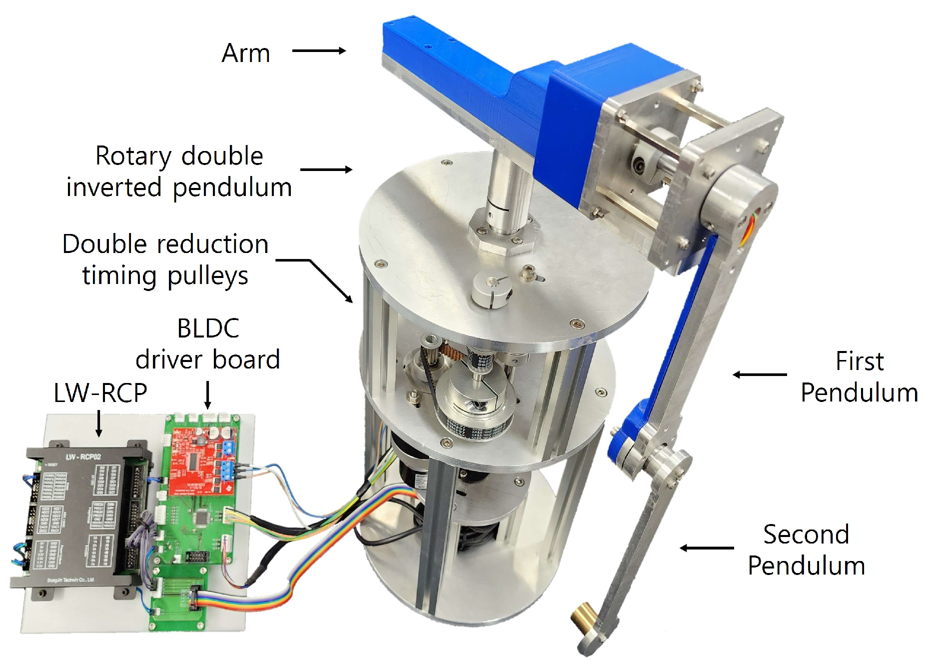
The project's homepage contains a wealth of resources, including MATLAB scripts and Simulink models for design and, most importantly, performance verification.

This resource is your practical guide. When you are ready to work on your specific pendulum problem, you can use the provided files like Edukit_Full_State_Inverted_Mode_LQR_Design.m to design a controller and Edukit_Full_State_Performance_Measurement.m to simulate and plot its response, just as we've discussed.

Conclusion

Today, we closed the loop on the design process. After calculating a gain matrix K, it's essential to simulate the system to verify that the real-world performance matches your design goals.

Key Takeaways:

• A closed-loop system model can be formulated to include a reference input, allowing simulation of tracking performance.
• Simulation tools like MATLAB's step or lsim, or numerical integrators like ode45, are used to plot the system's time-domain response.
• By analyzing these plots, you can verify performance metrics like settling time and overshoot.
• There is a critical trade-off between aggressive performance (fast response) and control effort/robustness. Placing poles very far into the left-half plane leads to high-gain controllers that can be sensitive to noise and nonlinearities.
• Always test your linear controller design on a nonlinear model if one is available, as it provides a more realistic performance preview.

Preview of the Next Lesson:
Our entire design for state feedback relies on one critical assumption: that we have access to all state variables in the vector $x$ for our feedback law $u=-Kx$. What if we don't? For the pendulum, you might have a sensor for the arm angle and the pendulum angle, but what about their velocities? Measuring velocity directly is often difficult or expensive.

In the next module, we will tackle this exact problem by learning how to estimate the states we cannot measure. This will lead us to the design of Luenberger observers, a powerful tool for reconstructing the full state vector from only the available output measurements.