Support Vector Machines for Classification

1. The Core Idea: The Maximal Margin Classifier

Imagine you have data points belonging to two different classes on a 2D plot. Your goal is to draw a line that separates them. As you might guess, there isn't just one line that can do the job; there could be infinitely many. So, which one is the best?

The core idea of an SVM is to choose the line that is as far as possible from the nearest data points of both classes. Think of it as drawing the widest possible "street" between the two groups of points. The line running down the middle of this street is our optimal decision boundary.

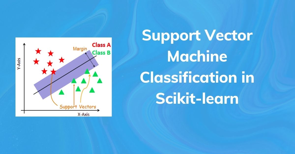
Let's formalize these terms:

• Hyperplane: This is the technical name for the decision boundary. In a 2D space, it's a line. In a 3D space, it's a flat plane. In spaces with more than three dimensions, we call it a hyperplane.
• Margin: This is the distance from the hyperplane to the closest points on either side. SVMs aim to maximize this margin. A wider margin suggests a more confident and robust model that is likely to generalize well to new data.
• Support Vectors: These are the data points that lie closest to the hyperplane, right on the edge of the margin. They are the most critical data points because they alone determine the position and orientation of the hyperplane. If you were to move any other point, the hyperplane wouldn't change. But if you move a support vector, the hyperplane will likely have to adjust.

This maximal margin approach seems great, but what happens if the data isn't perfectly separable? What if there are outliers?

2. Handling Imperfect Data: The Soft Margin Classifier

Real-world data is rarely perfect. Often, classes overlap, or there are outlier points that lie on the "wrong" side of where a clean boundary would be. A strict maximal margin classifier (also called a hard margin SVM) would fail in these situations or produce a very poor boundary.

To solve this, we use a soft margin SVM. This approach allows some data points to be misclassified or to fall inside the margin, but it adds a penalty for each of these violations. This creates a balance—a trade-off—between two goals:

1. Keeping the margin as wide as possible.
2. Minimizing the number of margin violations.

This is another example of the bias-variance tradeoff we've discussed before. A very strict model (high C) might have low bias but high variance (overfitting to the training data, including its noise). A more flexible model (low C) might have higher bias but lower variance (better generalization).

The degree of this trade-off is controlled by a hyperparameter, typically denoted as C.

In summary:

• A high C value puts a high penalty on misclassification. The SVM will try to classify as many examples correctly as possible, leading to a narrower margin and potentially overfitting.
• A low C value puts a lower penalty on misclassification. The SVM will prioritize a wider margin, even if it means misclassifying a few training points. This often leads to better generalization.

3. Handling Non-Linear Data: The Kernel Trick

So far, we've only considered data that is more or less linearly separable. But what if our data looks like this, where no straight line could ever separate the classes effectively?

This image from GeeksForGeeks shows a dataset where the classes are arranged in concentric circles. A linear hyperplane cannot separate these classes.

This is where SVMs truly shine, thanks to a powerful mathematical idea called the kernel trick.

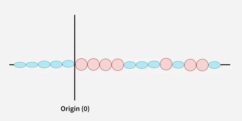
The core idea is this: if we can't separate the data in its current dimension, let's project it into a higher dimension where it does become linearly separable.

The "trick" is that we can do this without ever actually calculating the new coordinates of the points in the higher-dimensional space. Kernel functions allow us to compute the relationships between points as if they were in that higher space, which is computationally much cheaper.

Common SVM Kernels

You don't need to invent these transformation functions yourself. SVMs come with several standard kernels you can choose from. Let's look at the most common ones.

Here's a quick summary of the key kernels and their hyperparameters:

• Linear Kernel: For linearly separable data. The main hyperparameter is C.
• Polynomial Kernel: For data with a curved boundary. Hyperparameters include C, degree of the polynomial, and gamma.
• RBF (Radial Basis Function) Kernel: The most popular and flexible choice. It can create complex, non-linear boundaries. Its key hyperparameters are C and gamma.
  • gamma defines how much influence a single training example has. A low gamma means a point has far-reaching influence (smoother boundary), while a high gamma means influence is very local (tighter, more complex boundary).

4. Implementing SVM in Python with scikit-learn

Now for the practical part. Implementing an SVM in Python is straightforward using the scikit-learn library. The main class is SVC (Support Vector Classifier) from the sklearn.svm module.

The article we've been referencing has a great, simple code example that not only trains the model but also visualizes the result, including the hyperplane, margin, and support vectors.

The key line of code is instantiating the classifier:
model = SVC(kernel='rbf', C=1.0, gamma='auto')

Here, you can specify:

• kernel: The kernel to use (e.g., 'linear', 'poly', 'rbf').
• C: The regularization parameter.
• gamma: The kernel coefficient for 'rbf' and 'poly'.

You would then train the model just like any other scikit-learn classifier: model.fit(X_train, y_train).

Conclusion

Great work! You've now learned about another cornerstone algorithm in machine learning. Unlike ensemble methods that combine many models, SVMs focus on finding a single, optimal separating boundary.

Key Takeaways:

• An SVM's goal is to find a hyperplane that creates the maximum margin between two classes.
• The data points that define this hyperplane are called support vectors.
• The soft margin approach, controlled by the C hyperparameter, allows SVMs to handle noisy and overlapping data by trading off margin width against misclassification errors.
• The kernel trick enables SVMs to solve complex, non-linear problems by implicitly mapping data to a higher-dimensional space. The RBF kernel, controlled by gamma, is a powerful and popular default choice.

Preview of the Next Lesson:
So far in this course, all the machine learning we have done has been supervised learning—where we have labeled data (e.g., we know which tumor is benign or malignant). In our next lesson, we will venture into unsupervised learning, where the data has no labels. We will start with a fundamental clustering algorithm: k-means clustering, which is used to automatically discover groups in your data.