Hello! Welcome to the fifth lesson in our "Mathematical Foundations: Linear Algebra" module.
In our previous lesson, we explored determinants and matrix inverses. We learned that for a square matrix, a non-zero determinant signals that the matrix has an inverse and that a corresponding linear system has a unique solution. This was a powerful insight, but it was limited to square matrices.
Today, we'll introduce a concept that applies to any matrix, square or not: the rank. The rank gives us a deeper understanding of a matrix's structure and the nature of the solutions to linear systems. This lesson directly addresses the learning outcome: Determine the rank of a matrix using row reduction techniques. We will see how the Gaussian elimination process you learned a few lessons ago is the key tool for finding a matrix's rank.
1. What is the Rank of a Matrix?
At its core, the rank of a matrix is the number of linearly independent rows it contains. You can think of this as the number of "unique" or "non-redundant" rows. If one row can be created by combining other rows (e.g., Row 3 = 2 * Row 1 + Row 2), it's considered redundant or linearly dependent. The rank essentially tells us the "true" dimension of the vector space spanned by the rows of the matrix.
While this definition is conceptually important, it doesn't give us a straightforward way to calculate the rank. For that, we need a standard form to which we can reduce any matrix. This standard form is called Row Echelon Form.
2. Row Echelon Form (REF)
The most common method to find the rank of a matrix is to first transform it into Row Echelon Form (REF) using the row operations you're already familiar with. A matrix is in REF if it satisfies two simple rules.
The following video provides a clear explanation of what REF is and why it's useful.
Watch this short video from The Complete Guide to Everything to understand the two essential rules that define Row Echelon Form. It also directly connects this form to the concept of rank.
Watch from the beginning until 03:51. Focus on: The two rules for a matrix to be in REF (00:00 - 02:49). The definition of 'pivots' and how the rank is simply the number of pivots, which is the same as the number of non-zero rows in REF (02:49 - 03:51).
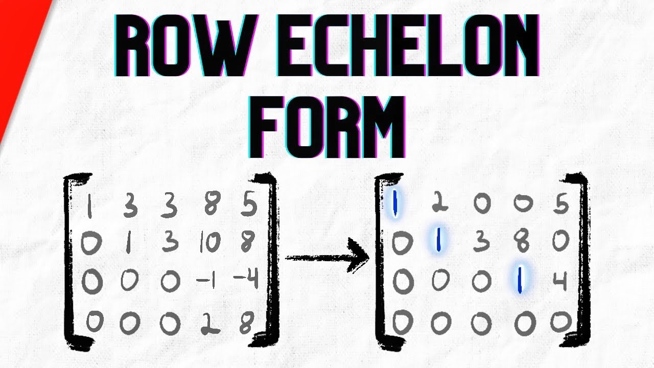
To summarize the key points from the video, a matrix is in Row Echelon Form if:
- All rows consisting entirely of zeros are at the bottom of the matrix.
- The first non-zero entry from the left in each non-zero row (called the leading entry or pivot) is to the right of the leading entry of the row above it.
This structure creates a "staircase" pattern in the matrix.
3. Calculating the Rank using Row Reduction
Now we can state the primary method for finding the rank, which connects all these ideas:
The rank of a matrix is the number of non-zero rows in its Row Echelon Form.
The process of transforming a matrix into REF is called row reduction or Gaussian Elimination. You've already used this algorithm to solve systems of linear equations. Now, we'll use it for a different purpose: finding the rank.
The following text provides a formal definition of rank and a step-by-step description of the Gaussian Algorithm for row reduction.
SYS-0030: Gaussian Elimination and Rank
This article from Ximera provides a formal definition of rank and outlines the Gaussian Algorithm for achieving row echelon form.
First, read the section titled 'Rank'. It formally defines rank as the number of non-zero rows in any row-echelon form. Next, read the section 'Gaussian and Gauss-Jordan Elimination', specifically focusing on the steps of the 'Gaussian Algorithm'. You don't need to memorize it, but understand the general strategy: identify a pivot, use it to create zeros below it, and then repeat the process on the sub-matrix below.
The algorithm essentially works as follows:
- Identify the first column with a non-zero entry. This is your first pivot column.
- Use row swaps if necessary to move a non-zero entry to the top of this column. This is your first pivot.
- Use row operations to make all entries below this pivot zero.
- Ignore the pivot's row and repeat the process on the remaining sub-matrix until the entire matrix is in REF.
Let's watch a video that walks through this entire process.
How to Find the Rank of a Matrix (with echelon form) | Linear Algebra
This video from Wrath of Math demonstrates the full process: taking a matrix, performing row operations to get it into row echelon form, and then counting the non-zero rows to find the rank.
Watch these two segments: First, watch from 00:22 to 01:17 to see the basic idea applied to two matrices. Then, watch the detailed walkthrough of a larger matrix from 02:08 to 03:24. Observe how row operations are used systematically to create zeros below the pivots.
Test your understanding!
Let's find the rank of the following matrix :
Follow the Gaussian elimination steps to transform it into Row Echelon Form and then state its rank.
Show answer
Step 1: The pivot in the first row is 1. We use it to create zeros in the column below it.
- Replace Row 2 with .
- Replace Row 3 with .
Step 2: The matrix is not yet in REF. We look at the sub-matrix below the first row. The pivot in the second row is 1. We use it to create a zero below it.
- Replace Row 3 with .
Step 3: The matrix is now in Row Echelon Form. We count the number of non-zero rows. There are two non-zero rows (Row 1 and Row 2).
Therefore, the rank of A is 2.
Conclusion
In this lesson, you learned how to determine one of the most fundamental properties of a matrix: its rank. You now understand that rank is not just an abstract number, but a measure of the "dimensionality" or "information content" of a matrix.
Key Takeaways:
- The rank of a matrix is the number of its linearly independent rows (or columns).
- To find the rank, we use row reduction (Gaussian elimination) to convert the matrix into Row Echelon Form (REF).
- The rank is simply the number of non-zero rows in the resulting REF matrix.
- This method works for any matrix, regardless of its size or whether it is square.
In our last two lessons on determinants and rank, we've been analyzing the properties of matrices. In the next lesson, we will explore eigenvalues and eigenvectors. These are special vectors whose direction is unchanged when a matrix transformation is applied. Understanding them is crucial for many applications in data science, such as Principal Component Analysis (PCA), which you'll encounter later in your studies. The concept of rank will be helpful, as it relates to the number of non-zero eigenvalues a matrix has.