Fibonacci with Memoization and Tabulation

Introduction

In our previous lesson, we established the core principles of Dynamic Programming (DP). You learned that a problem is a good candidate for DP if it has optimal substructure and, crucially, overlapping subproblems. We saw how a naive recursive solution for the Fibonacci sequence becomes incredibly slow because it repeatedly calculates the same values, a classic sign of overlapping subproblems.

Today, we'll move from theory to practice. You will learn the two primary techniques for implementing a DP solution to fix this inefficiency. Your learning outcome for this lesson is to: Solve the Fibonacci sequence problem using both memoization (top-down) and tabulation (bottom-up) DP.

By the end of this lesson, you will be able to write efficient Python code for the Fibonacci sequence and understand the trade-offs between these two powerful DP approaches. This is a fundamental skill that you'll build upon to solve more complex DP problems required for the GATE exam.

First, let's visualize the two paths we're about to take.

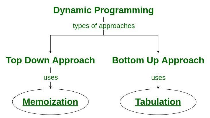
The Problem Revisited: Inefficient Recursion

As a quick refresher, let's look at the simple, but inefficient, recursive function for the Fibonacci sequence.

def fib_recursive(n):
    # Base cases
    if n <= 1:
        return n
    # Recursive step with overlapping subproblems
    return fib_recursive(n - 1) + fib_recursive(n - 2)

# Trying to calculate fib_recursive(40) would take a very long time!

As we discussed, the issue is that fib_recursive(n-1) and fib_recursive(n-2) lead to a tree of function calls with many redundant branches. For example, calculating fib_recursive(5) ends up calculating fib_recursive(2) three separate times.

This leads to an exponential time complexity of $O(2^n)$. Now, let's see how DP solves this.

1. Memoization: The Top-Down Approach

Memoization is a technique where you store the results of expensive function calls and return the cached result when the same inputs occur again. It's like adding a memory to our recursive function.

This is called a top-down approach because you start with the original problem (e.g., fib(n)) and break it down recursively. The magic happens when a subproblem is encountered for the second time; instead of re-computing, you just look up the answer.

To understand how to convert a recursive solution into a memoized one, let's watch a detailed explanation.

Steps to Implement Memoization:

As the video explained, you can convert almost any pure recursive function to a memoized one with these steps:

1. Create a cache: Create a data structure (like an array or a dictionary) to store the results of subproblems. Initialize it with a sentinel value (e.g., -1) to indicate that a subproblem hasn't been solved yet.
2. Check the cache: At the beginning of your function, before any computation, check if the solution for the current state is already in the cache. If it is, return the cached value immediately.
3. Store the result: If the solution was not in the cache, compute it recursively as before. Then, just before returning the result, store it in the cache.

Here is what this looks like in Python:

# A cache (or dp array) to store Fibonacci numbers
# We can initialize it with -1 to indicate 'not yet computed'
n = 10
dp = [-1] * (n + 1)

def fib_memo(n):
    # Base cases
    if n <= 1:
        return n

    # 1. Check if the result is already in our cache
    if dp[n] != -1:
        return dp[n]

    # 2. If not, compute it recursively
    result = fib_memo(n - 1) + fib_memo(n - 2)
    
    # 3. Store the result in the cache before returning
    dp[n] = result
    return result

print(f"The {n}th Fibonacci number is: {fib_memo(n)}")
# This would now calculate fib(40) almost instantly.

Complexity Analysis (Memoization)

• Time Complexity: $O(n)$. Each Fibonacci number from 2 to n is computed only once. Subsequent calls are $O(1)$ lookups.
• Space Complexity: $O(n)$. This comes from two sources: the size of our dp array ($O(n)$) and the depth of the recursion stack, which can go up to n in the worst case ($O(n)$).

2. Tabulation: The Bottom-Up Approach

Tabulation takes the opposite approach. Instead of starting from n and going down, it starts from the base cases and builds the solution iteratively up to n. It fills a "table" (usually an array) from the beginning.

This is called a bottom-up approach because you solve the smallest subproblems first and use their results to build up solutions to larger subproblems. For Fibonacci, this is very intuitive: calculate fib(2), then fib(3), then fib(4), and so on, until you reach fib(n).

To see how this is done, let's go back to our guide.

Steps to Implement Tabulation:

1. Create a table: Create a dp array of size n+1 to store the results.
2. Initialize base cases: Manually fill in the solutions for the base cases in the table (e.g., dp[0] = 0, dp[1] = 1).
3. Iterate and fill: Loop from the first unsolved subproblem up to n. In each iteration, calculate dp[i] using the already-computed values in the table (dp[i-1] and dp[i-2]).
4. Return the final answer: The solution to the original problem is the last value computed: dp[n].

Here's the Python implementation:

def fib_tabulation(n):
    # Handle base cases for n=0 and n=1
    if n <= 1:
        return n

    # 1. Create the table
    dp = [0] * (n + 1)

    # 2. Initialize base cases
    dp[1] = 1

    # 3. Iterate from 2 to n and fill the table
    for i in range(2, n + 1):
        dp[i] = dp[i - 1] + dp[i - 2]
    
    # 4. The answer is at the end of the table
    return dp[n]

n = 10
print(f"The {n}th Fibonacci number is: {fib_tabulation(n)}")

Complexity Analysis (Tabulation)

• Time Complexity: $O(n)$. We simply loop from 2 to n once.
• Space Complexity: $O(n)$. We use an array of size n+1 to store the results. Notice that unlike memoization, there is no extra space used by a recursion stack.

3. Space Optimization

If you look closely at the tabulation loop, you'll see a key detail: to compute dp[i], we only need dp[i-1] and dp[i-2]. We don't need dp[i-3], dp[i-4], etc. So, why are we storing the entire array?

We can optimize the space complexity from $O(n)$ down to $O(1)$ by only keeping track of the last two values.

Let's see how this final optimization is done.

Here's the space-optimized code in Python:

def fib_optimized(n):
    if n <= 1:
        return n
    
    # We only need the previous two numbers
    prev2 = 0  # Represents fib(i-2)
    prev1 = 1  # Represents fib(i-1)
    
    # Loop from 2 to n
    for _ in range(2, n + 1):
        current = prev1 + prev2
        # Update pointers for the next iteration
        prev2 = prev1
        prev1 = current
        
    return prev1 # prev1 holds the final fib(n)

n = 10
print(f"The {n}th Fibonacci number is: {fib_optimized(n)}")

Complexity Analysis (Space-Optimized)

• Time Complexity: $O(n)$. The loop still runs n-1 times.
• Space Complexity: $O(1)$. We only use a few variables (prev2, prev1, current), regardless of the size of n. This is the most efficient solution for this problem.

Conclusion

Congratulations! You've successfully implemented your first Dynamic Programming problem using three different approaches. This is a huge step in building your algorithmic toolkit.

Key Takeaways:

• Memoization (Top-Down): A recursive approach that adds a cache to avoid recomputing subproblems. It's often more intuitive to write if you already have a recursive solution.
  • Time: $O(n)$ | Space: $O(n)$ (for cache + recursion stack)
• Tabulation (Bottom-Up): An iterative approach that builds the solution from the smallest subproblems up. It avoids recursion overhead.
  • Time: $O(n)$ | Space: $O(n)$ (for the table)
• Space Optimization: For problems like Fibonacci, where the solution only depends on a few previous results, we can optimize the tabulation approach to use constant space.
  • Time: $O(n)$ | Space: $O(1)$

Preview of the Next Lesson:

We've now seen how DP thoroughly explores subproblems to guarantee an optimal solution. In our next lesson, we will explore a different algorithmic paradigm: Greedy Algorithms. We will learn how a greedy algorithm makes the "best-looking" choice at each step, hoping to find a global optimum. We will contrast this with DP and learn to identify when a simpler, faster greedy approach is sufficient by applying it to the Activity Selection problem.