Greedy Algorithms: Activity Selection

Introduction

In our last lesson, we explored Dynamic Programming (DP), a powerful technique for solving complex optimization problems. You learned that DP works by breaking a problem down into smaller overlapping subproblems and exhaustively solving them (using memoization or tabulation) to guarantee a globally optimal solution.

Today, we'll examine a different, often simpler, algorithmic paradigm: Greedy Algorithms. Your learning outcome for this lesson is to: Describe the greedy algorithm paradigm and apply it to solve the Activity Selection problem.

Unlike DP, which explores many possibilities, a greedy algorithm makes the choice that seems best at the current moment and sticks with it, hoping this series of "locally optimal" choices leads to a "globally optimal" solution. We'll explore this core idea, learn when it's appropriate, and apply it to a classic problem that often appears in competitive programming and exams like GATE.

What is a Greedy Algorithm?

A greedy algorithm builds a solution piece by piece. At each step, it chooses the option that offers the most immediate and obvious benefit, without considering the future consequences of that choice. It's like climbing a hill by always taking the steepest path up from where you are, hoping it leads you to the absolute highest peak.

As you saw, the greedy approach is simpler and faster, but it comes with a big risk: it might not find the best overall solution. It only works for problems with a special property called the greedy choice property, which means a locally optimal choice is always part of some globally optimal solution.

Key Characteristics

• Locally Optimal Choices: It makes the best choice available at each step.
• Irrevocable: Once a choice is made, it's never reconsidered.
• Fast: They are generally very efficient, often with time complexities like $O(n)$ or $O(n\log n)$.
• Not Always Optimal: The main challenge is proving that the greedy strategy actually leads to a globally optimal solution for a given problem.

The Activity Selection Problem

Let's apply this paradigm to a famous problem where a greedy approach does work perfectly.

Problem Statement: You are given a set of n activities, each with a specific start time and finish time. You need to select the maximum number of activities that can be performed by a single person, assuming that a person can only work on one activity at a time.

For example, if you have these activities:

• Activity 1: Start 1, Finish 3
• Activity 2: Start 2, Finish 5
• Activity 3: Start 4, Finish 6

You can perform Activity 1 and Activity 3 (total 2 activities). You cannot perform Activity 1 and 2, because they overlap. The goal is to find the largest possible set of non-overlapping activities.

Crafting a Greedy Strategy

How would you greedily choose which activity to do next? Here are a few intuitive ideas:

1. Earliest Start Time First: Pick the activity that starts earliest. This seems logical, but what if that activity runs for a very long time and blocks many other shorter activities? This strategy can fail.
2. Shortest Duration First: Pick the activity with the shortest duration (finish time - start time). This also seems plausible, but a very short activity might be scheduled right in the middle of a time slot, preventing you from picking two other activities on either side of it. This can also fail.
3. Earliest Finish Time First: Pick the activity that finishes earliest.

Let's analyze these ideas more formally.

As the video explains, the winning strategy is to always choose the activity that finishes earliest. The intuition is that this frees up your time as quickly as possible, thereby maximizing the opportunity to schedule more activities later.

The Algorithm: Step-by-Step

Here is the formal greedy algorithm for the Activity Selection Problem:

1. Sort the activities in ascending order based on their finish times.
2. Select the first activity from the sorted list and add it to your result set.
3. Iterate through the rest of the sorted activities (from the second one onwards). For each activity, if its start time is greater than or equal to the finish time of the previously selected activity, select this activity and add it to your result set.

Let's see this in action.

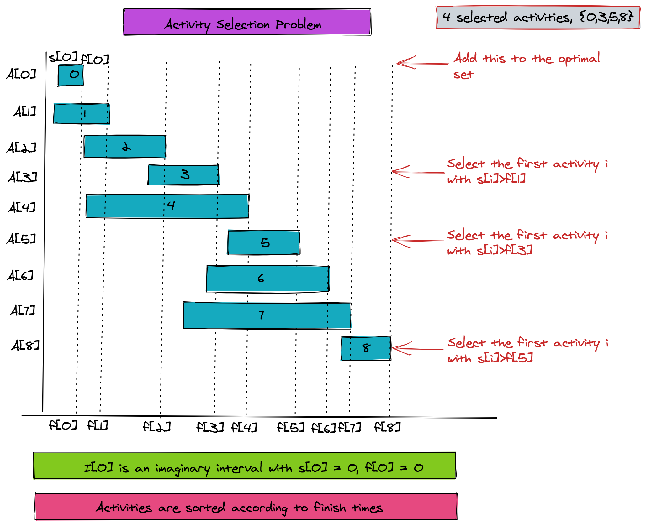
Why Does This Work?

The correctness of this algorithm can be proven. The core idea is that by picking the activity that finishes first, you are making a "safe" move. This choice is guaranteed to be part of some optimal solution.

For a brief logical proof, watch the next segment of the video.

Python Implementation

Now, let's translate this algorithm into Python code. Since you're starting your programming journey, we'll look at a clear implementation that handles the data structures and sorting correctly.

The Python code you just studied uses a lambda function for sorting: sorted(activities, key=lambda activity: activity[1]). This is a common and powerful Python feature. It creates a small, anonymous function that tells the sorted function to look at the element at index 1 (the finish time) of each activity tuple when comparing items.

Complexity Analysis

• Time Complexity: The most time-consuming step is sorting the activities, which takes $O(n\log n)$ time. The subsequent loop to select activities takes only $O(n)$ time. Therefore, the overall time complexity is dominated by the sorting step: $O(n\log n)$.
• Space Complexity: If you modify the input array in place, the space complexity can be $O(1)$. If you create a new data structure to store the sorted activities, it is $O(n)$.

Conclusion

In this lesson, we introduced the greedy algorithm paradigm and contrasted it with the more exhaustive Dynamic Programming approach. You learned that greedy algorithms make locally optimal choices at each step, a strategy that is fast and simple but only works for certain optimization problems.

Key Takeaways:

• Greedy Paradigm: Build a solution by making a sequence of irrevocable choices that seem best at the moment.
• Greedy vs. DP: DP solves overlapping subproblems to guarantee a global optimum. Greedy makes a single "best" choice and moves on, which is faster but not always correct.
• Activity Selection Problem: A classic problem that can be optimally solved with a greedy strategy.
• The Winning Strategy: Sort activities by their finish times and pick the next compatible activity. This always yields a maximum set of activities.

Preview of the Next Lesson:

Many of the most famous algorithms, including greedy ones like Dijkstra's or Kruskal's, operate on graphs. Before we can study them, we need to understand how to represent graphs in code. In the next lesson, we will cover the fundamental ways to do this: "Implement graph representations (adjacency list, adjacency matrix) in Python." This will be a critical building block for much of the rest of the course.