Handling Missing Values and Feature Scaling

A Crucial First Principle: Splitting Before Preprocessing

Before we dive in, let's establish a golden rule that connects to our last lesson: Any data preprocessing step that involves learning parameters from the data must be done after splitting the data.

Why? Imagine you calculate the average value of a feature to fill in missing entries. If you use the entire dataset (before splitting), you have calculated an average that includes information from your validation and test sets. This information has now "leaked" into your training set. Your model's performance will be artificially inflated because it has indirectly learned something about the data it's supposed to be tested on.

The correct workflow is:

1. Split data into training, validation, and test sets.
2. Learn the preprocessing parameters (like the mean for imputation or the min/max for scaling) only from the training set.
3. Apply (or "transform") all three sets (training, validation, and test) using these learned parameters.

We will keep this rule in mind throughout the lesson.

Part 1: Handling Missing Values

Real-world datasets are often messy and incomplete. Values might be missing because they weren't recorded, were lost, or simply don't exist. Most machine learning algorithms in scikit-learn cannot function when they encounter missing values (often represented as NaN, or "Not a Number").

Identifying Missing Values

In pandas, you can quickly check for missing values in your DataFrame. If you have a DataFrame named df, you can run:

# This will show you the count of missing values in each column
df.isnull().sum()

Strategies for Handling Missing Values

There are two main approaches: deletion and imputation.

1. Deletion
You could simply delete rows (df.dropna()) or entire columns that contain missing values.

• Pros: It's simple.
• Cons: This is usually a bad idea. You risk throwing away valuable information. If a column has many missing values but is highly predictive, deleting it hurts your model. If many rows have at least one missing value, you could end up with a tiny dataset.

2. Imputation
Imputation is the process of filling in missing values. This is the preferred approach. The key is to make a reasonable guess about what the missing value might have been.

Common imputation strategies include:

• Mean: Replace missing values with the average of the column. Best for normally distributed data.
• Median: Replace missing values with the median of the column. This is more robust to outliers and a good default choice for numerical data.
• Most Frequent (Mode): Replace missing values with the most common value. This is the go-to method for categorical (non-numeric) features.
• Constant: Replace missing values with a fixed value, like 0, "missing", or "unknown". This can be useful if the fact that a value is missing is itself informative.

Practical Imputation with Scikit-Learn's SimpleImputer

The best way to learn this is to see it in action. The following video demonstrates how to use scikit-learn's SimpleImputer, which is the standard tool for this job.

As you saw, the process is straightforward:

1. Import SimpleImputer.
2. Create an imputer object, specifying your chosen strategy.
3. Fit the imputer on your training data (imputer.fit(X_train)).
4. Transform your training, validation, and test data (imputer.transform(X_train), imputer.transform(X_val), etc.).

Part 2: Feature Scaling

Now, let's look at another common issue. Imagine you have a dataset with two features: age (ranging from 20-70) and salary (ranging from 50,000-2,000,000). Many ML algorithms, particularly those that rely on distances or gradients, will be biased towards the salary feature simply because its numbers are much larger. Its scale dominates the age feature.

Feature scaling puts all features onto a similar scale so that they contribute more equally to the model's training process.

Why and When to Scale?

This next short video explains the intuition behind why scaling is so important for certain algorithms.

As the video and the following article explain, scaling is crucial for some models but not for others.

In short:

• Scale your data for: Linear/Logistic Regression, Neural Networks, SVM, K-NN, K-Means, and PCA.
• You don't need to scale for: Tree-based algorithms like Decision Trees, Random Forests, and Gradient Boosting.

Types of Feature Scaling

There are two primary methods of feature scaling you must know: Standardization and Normalization.

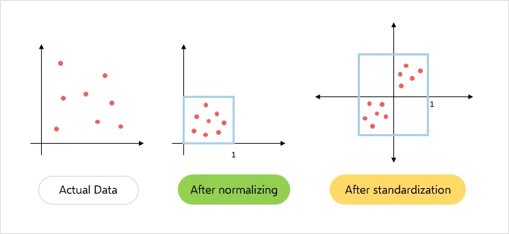
1. Standardization (Z-score Scaling)
Standardization rescales the data to have a mean of 0 and a standard deviation of 1.

• Formula: $X_{feature}^{\prime }=\frac{X_{feature}-{\mu }_{feature}}{{\sigma }_{feature}}$
• Intuition: It tells you how many standard deviations away from the mean each data point is.
• When to use: This is the most common scaling method and is a great default choice. It is less sensitive to outliers than normalization.
• Scikit-learn: StandardScaler

2. Normalization (Min-Max Scaling)
Normalization rescales the data to a fixed range, usually [0, 1].

• Formula: $X_{feature}^{\prime }=\frac{X_{feature}-\min (X_{feature})}{\max (X_{feature})-\min (X_{feature})}$
• Intuition: It squeezes all your data points into a specific range.
• When to use: Useful for algorithms that expect data in a bounded range (like some neural networks) or when you need your features on the exact same scale. It's very sensitive to outliers.
• Scikit-learn: MinMaxScaler

To see the practical implementation and a more detailed comparison, please review the following sections of the blog post we looked at earlier.

Conclusion

Congratulations! You have now learned how to perform two of the most critical steps in the data preprocessing pipeline. Clean, well-prepared data is the foundation of any successful machine learning project.

Key Takeaways:

• Always split your data before you preprocess it to avoid data leakage.
• Handle missing values using imputation (SimpleImputer), typically with the median or most_frequent strategy.
• Apply feature scaling for algorithms sensitive to feature magnitudes (e.g., K-NN, SVM, Linear Regression).
• Standardization (StandardScaler) is a robust default choice for scaling, centering data at mean 0 with a standard deviation of 1.
• Normalization (MinMaxScaler) scales data to a fixed range (e.g., [0, 1]) but is sensitive to outliers.
• Always fit your imputer and scaler only on the training data, and then use them to transform the training, validation, and test sets.

Preview of the Next Lesson:
We have organized our data with train/val/test splits and cleaned it by handling missing values and applying scaling. We are finally ready to build our first model! In the next lesson, we will dive into one of the simplest yet most important models in machine learning: you will learn to describe the mathematical formulation of a simple linear regression model.