Understanding Simple Linear Regression: The Equation

Hello! Welcome to the fourth lesson in the "Foundations of Machine Learning" module.

In our last lesson, we focused on essential data preprocessing techniques: handling missing values and scaling our features. You learned that scaling is particularly important for algorithms like linear regression. Now that we know how to prepare our data, it's time to build our first predictive model.

This lesson dives into the fundamental building block of regression models. Your learning outcome is to describe the mathematical formulation of a simple linear regression model. We will move from the simple idea of drawing a line through data points to a precise mathematical equation that forms the basis of many advanced machine learning concepts. Understanding this is crucial for your GATE preparation and for building a solid foundation in data science.

1. The Goal: Modeling a Relationship

At its core, linear regression is about finding a linear relationship between two variables:

An independent variable (also called the input, feature, or predictor), which we'll denote as $X$ .
A dependent variable (also called the output, target, or response), which we'll denote as $Y$ .

The goal is to use the value of $X$ to predict the value of $Y$ . For example, we might want to predict a house's price ( $Y$ ) based on its size ( $X$ ).

To understand the core objectives and terminology of linear regression, let's start with a short introductory video.

Video 1: Introduction to Simple Linear Regression

This video from dataminingincae provides a clear introduction to the main goals of simple linear regression and defines the roles of dependent and independent variables.

Please watch the video from the beginning until 03:40. Focus on understanding: The two main objectives: establishing a relationship and forecasting. The definitions of the dependent variable (Y) and independent variable (X).

As the video explained, we are looking for a straight line that best represents the data. You might remember the equation of a line from school as $y = m x + c$ . In machine learning, we use slightly different notation, but the concept is exactly the same.

2. The Mathematical Formulation of the Model

The primary task in linear regression is to find the specific straight line that best "fits" our data. To do this, we need a formal equation.

The Hypothesis Function

In machine learning, the model we create is often called a hypothesis function, usually denoted as $h (x)$ . This function takes an input $x$ and outputs a predicted value, which we call $y^$ ("y-hat").

For simple linear regression, the hypothesis function is the equation of a line:

y^= θ_{0} + θ_{1} x

Let's break down the components:

$y^$ : The predicted value of the target variable.
$x$ : The input feature.
$θ_{0}$ (theta-zero): The intercept of the line. This is the predicted value of $y^$ when $x = 0$ . It's the "starting point" of our line on the y-axis.
$θ_{1}$ (theta-one): The slope or coefficient of the line. This value determines how much $y^$ changes for a one-unit increase in $x$ .

The terms $θ_{0}$ and $θ_{1}$ are the parameters of our model. The "learning" part of machine learning is the process of finding the optimal values for these parameters.

You will encounter different notations for this same equation in various resources. It's important to recognize them:

h(x) = θ₀ + θ₁x (Common in ML courses, like Andrew Ng's)
y = β₀ + β₁x (Common in statistics)
y = w₀ + w₁x (Here w stands for "weights," common in deep learning)
y = b + mx (Connects to classic algebra, where b is the bias/intercept)

All these equations represent the same simple linear model. We will primarily use the $θ$ notation.

Accounting for Real-World Noise: The Error Term

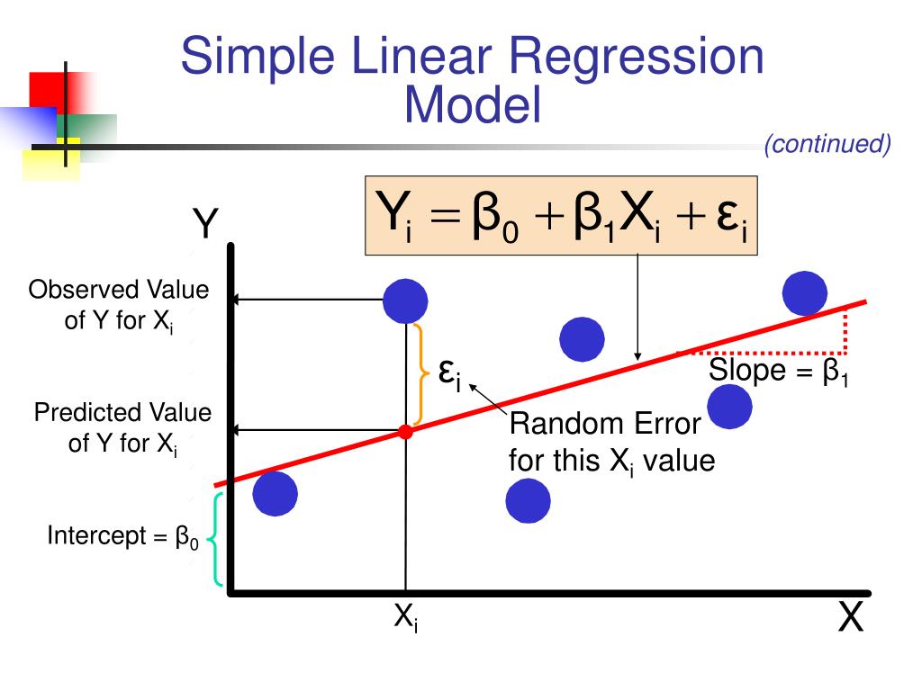
In the real world, data points rarely fall perfectly on a straight line. There's always some "noise" or variability that our model can't explain. To account for this, the full statistical model of linear regression includes an error term, denoted by $ϵ$ (epsilon).

The complete equation for an actual observed data point $y_{i}$ is:

y_{i} = θ_{0} + θ_{1} x_{i} + ϵ_{i}

Here:

$y_{i}$ is the actual, observed value for the i-th data point.
$θ_{0} + θ_{1} x_{i}$ is the model's predicted value ( $y^_{i}$ ).
$ϵ_{i}$ is the random error for that data point—the difference between the actual value and the predicted value on the line.

The image below provides an excellent visual breakdown of this equation.

Simple Linear Regression Model Visual Explanation — This diagram illustrates the components of the linear regression equation on a scatter plot. It clearly shows the intercept ($β_0$), the slope ($β_1$), an observed data point ($Y_i$), its predicted value on the line, and the random error ($ε_i$) as the vertical distance between them.

To see a practical interpretation of these parameters, let's return to the video.

Video 1: Introduction to Simple Linear Regression

This part of the video explains how the intercept, slope, and error term come together in a real-world model. It uses graphical examples to show how changing the parameters affects the line.

Please watch from 03:28 to 08:21. Pay attention to: How the intercept (β_0) shifts the line up or down. How the slope (β_1) changes the steepness and direction of the line. Why the error term (ε) is necessary to model real-world data that isn't perfectly linear.

3. Measuring How "Good" the Fit Is: The Cost Function

We now have a model, $y^= θ_{0} + θ_{1} x$ . But how do we find the best values for $θ_{0}$ and $θ_{1}$ ? We need a way to measure how well a particular line (defined by a specific $θ_{0}$ and $θ_{1}$ ) fits our data.

This is the job of the cost function (also called a loss function or objective function). The cost function quantifies the total error between our model's predictions ( $y^$ ) and the actual target values ( $y$ ) across the entire training dataset.

For linear regression, the most common cost function is the Mean Squared Error (MSE).

Let's formalize this. In a supervised learning problem, we have a training set of $m$ examples: ${(x^{(1)}, y^{(1)}), (x^{(2)}, y^{(2)}), \dots, (x^{(m)}, y^{(m)})}$ .
For each example $i$ , our prediction is $y^^{(i)} = θ_{0} + θ_{1} x^{(i)}$ .

The MSE cost function, denoted as $J (θ_{0}, θ_{1})$ , is defined as:

J (θ_{0}, θ_{1}) = \frac{1}{2 m} i = 1 \sum m (y^^{(i)} - y^{(i)})^{2}

Substituting our hypothesis function, we get:

J (θ_{0}, θ_{1}) = \frac{1}{2 m} i = 1 \sum m (θ_{0} + θ_{1} x^{(i)} - y^{(i)})^{2}

Let's dissect this formula:

$(θ_{0} + θ_{1} x^{(i)} - y^{(i)})$ : This is the error for a single training example $i$ , the vertical distance between the prediction and the actual value.
$(\dots)^{2}$ : We square the error. This does two things: it makes all errors positive (so they don't cancel each other out) and it penalizes larger errors more heavily.
$\sum_{i = 1}^{m} \dots$ : We sum up the squared errors for all $m$ training examples.
$\frac{1}{m}$ : We take the average of the squared errors.
$\frac{1}{2}$ : This is a mathematical convention. Multiplying by $\frac{1}{2}$ makes the derivative calculation (which we'll see in the next lesson) cleaner. It doesn't change the values of $θ_{0}$ and $θ_{1}$ that minimize the function.

The goal of our learning algorithm is to find the values of $θ_{0}$ and $θ_{1}$ that result in the smallest possible value for $J (θ_{0}, θ_{1})$ .

The following resource provides a clear walkthrough of framing the linear regression problem and introducing the cost function.

A Deep Dive into Linear Regression

This article from Towards AI introduces the standard notation used in machine learning and builds up the intuition for the cost function.

Please read sections 1 and 2, focusing on: Standard Notation: Understand the meaning of x, y, m, and (x^(i), y^(i)). Representing the Model: See how the linear model is represented. The Cost Function: Reinforce your understanding of why we need a cost function to measure model quality.

Test your understanding!

Suppose you have a tiny dataset of 2 training examples:

House size $x^{(1)} = 1000$ sq ft, Price $y^{(1)} = 200$ thousand
House size $x^{(2)} = 2000$ sq ft, Price $y^{(2)} = 400$ thousand

You want to test a model with parameters $θ_{0} = 50$ and $θ_{1} = 0.15$ .

Calculate the Mean Squared Error cost $J (50, 0.15)$ for this model on this dataset. (You can ignore the $\frac{1}{2}$ for this exercise, as it's just a scaling factor).

Show answer

First, let's calculate the predictions ( $y^$ ) for each data point:

$y^^{(1)} = θ_{0} + θ_{1} x^{(1)} = 50 + 0.15 \times 1000 = 50 + 150 = 200$
$y^^{(2)} = θ_{0} + θ_{1} x^{(2)} = 50 + 0.15 \times 2000 = 50 + 300 = 350$

Next, let's calculate the squared error for each data point:

Error 1: $(y^^{(1)} - y^{(1)})^{2} = (200 - 200)^{2} = 0^{2} = 0$
Error 2: $(y^^{(2)} - y^{(2)})^{2} = (350 - 400)^{2} = (- 50)^{2} = 2500$

Finally, calculate the Mean Squared Error (with $m = 2$ ).

Cost = \frac{1}{m} i = 1 \sum m (y^^{(i)} - y^{(i)})^{2} = \frac{1}{2} (0 + 2500) = 1250

The cost for this specific line is 1250. Our goal in the next lesson will be to find parameters that make this cost even lower.

Conclusion

In this lesson, we have formally defined our first machine learning model. This is a significant step! You've moved from an intuitive idea to a concrete mathematical structure.

Key Takeaways:

Simple linear regression models the relationship between an input $X$ and an output $Y$ using a straight line.
The model's prediction is given by the hypothesis function: $y^= θ_{0} + θ_{1} x$ .
$θ_{0}$ (intercept) and $θ_{1}$ (slope) are the model parameters that the algorithm learns from the data.
The full statistical model includes an error term $ϵ$ to account for noise: $y = θ_{0} + θ_{1} x + ϵ$ .
To find the best parameters, we need to minimize a cost function. The standard choice is the Mean Squared Error (MSE), which measures the average squared difference between predictions and actual values.

Preview of the Next Lesson:
We've defined our goal: find the $θ_{0}$ and $θ_{1}$ that minimize the cost function $J (θ_{0}, θ_{1})$ . But how do we do that? In the next lesson, you will learn to apply gradient descent to optimize the cost function of a linear regression model. This powerful optimization algorithm is the engine that drives the learning process for linear regression and many other models in machine learning.