Logistic Regression for Binary Classification

1. Why Not Linear Regression for Classification?

Before we dive into what logistic regression is, let's understand the problem it solves. We have a classification task where the output is categorical (e.g., 0 or 1). Your first thought might be: why can't we just use linear regression, which we already know?

While it seems plausible, linear regression is not suited for classification. The following video explains this very clearly.

As the video demonstrates, linear regression can produce outputs outside the 0-1 range and is sensitive to outliers in a way that is problematic for classification. We need a model that is specifically designed to output a probability between 0 and 1.

2. The Core Idea: The Sigmoid Function

Logistic regression elegantly solves this problem by adding a crucial step to the linear model. It first calculates a linear combination of the input features (just like linear regression) and then passes this result through a special function called the sigmoid (or logistic) function.

The sigmoid function takes any real number and "squashes" it into the range between 0 and 1.

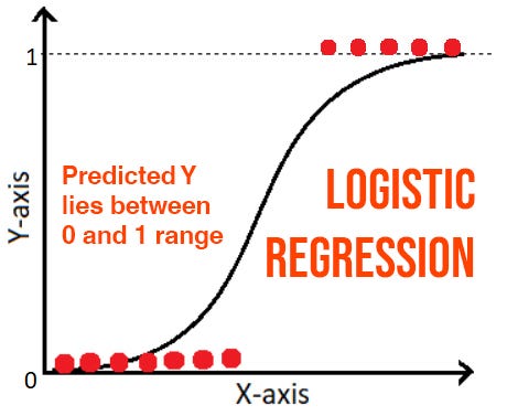
The mathematical formula for the linear part and the sigmoid transformation is:

1. Linear Step: Calculate $z$, which is a linear combination of features $X$ with weights $w$ and a bias $b$. $$z=w\cdot X+b$$
2. Sigmoid Step: Apply the sigmoid function, $\sigma (z)$, to get the predicted probability, $p$. $$p=\sigma (z)=\frac{1}{1+e^{-z}}$$

The resulting value, $p$, is the estimated probability that the output is "1". For example, if our model outputs $p=0.8$, it's predicting an 80% chance that the instance belongs to class 1.

To make a final classification (0 or 1), we use a decision threshold, which is typically 0.5.

• If $p\ge 0.5$, we predict class 1.
• If $p<0.5$, we predict class 0.

This threshold creates a linear decision boundary that separates the two classes in the feature space.

For a deeper look at the mathematics and the role of the sigmoid function, the following video and article are very helpful.

3. Implementing Logistic Regression with scikit-learn

Now, let's put this theory into practice. As with other algorithms, scikit-learn makes implementing logistic regression straightforward. The process follows the standard steps you've learned: import, instantiate, fit, and predict.

The next segment of the codebasics video provides a complete walkthrough of implementing logistic regression in Python to solve a binary classification problem.

The code to implement logistic regression is very concise. For example, using the breast cancer dataset, the core logic is just a few lines:

from sklearn.datasets import load_breast_cancer
from sklearn.linear_model import LogisticRegression
from sklearn.model_selection import train_test_split
from sklearn.metrics import accuracy_score

# 1. Load and split data
X, y = load_breast_cancer(return_X_y=True)
X_train, X_test, y_train, y_test = train_test_split(X, y, test_size=0.20, random_state=23)

# 2. Create and train the model
# max_iter is increased to ensure the model converges
clf = LogisticRegression(max_iter=10000, random_state=0)
clf.fit(X_train, y_train)

# 3. Make predictions and evaluate
y_pred = clf.predict(X_test)
acc = accuracy_score(y_test, y_pred)
print(f"Model accuracy: {acc:.2f}")

# Output: Model accuracy: 0.96

This example is also shown in the GeeksForGeeks article in section 4.

To get a more in-depth guide on the implementation details and the various parameters you can tune in scikit-learn's LogisticRegression class, the following resource is excellent.

4. Model Training and Evaluation

How does the model "learn" the best weights ($w$) and bias ($b$)? In the linear regression lesson, you saw that gradient descent was used to minimize the Mean Squared Error (MSE). Logistic regression uses a similar process but with a different cost function called Log Loss (or Binary Cross-Entropy). The goal is to find the parameters that minimize this log loss, which effectively maximizes the probability of the model assigning the correct labels to the training data.

After training, you can evaluate the model. The most straightforward metric is accuracy, which you can get with the .score() method. You can also see the predicted probabilities for each class using .predict_proba().

While accuracy is a good start, other metrics like the confusion matrix, precision, and recall give a more complete picture of a classifier's performance. We'll explore these in detail in the next module, but the Real Python article you read gives you a first look at them.

Conclusion

You have now learned how to implement logistic regression, a cornerstone algorithm for binary classification. It serves as a powerful bridge between the simple linear models and more complex classification techniques.

Key Takeaways:

• Logistic regression is a parametric algorithm for classification, not regression.
• It works by passing a linear combination of inputs through a sigmoid function to produce an output between 0 and 1, which is interpreted as a probability.
• A decision threshold (usually 0.5) is used to convert this probability into a final class prediction (0 or 1).
• The model is trained by finding the parameters that minimize a cost function called log loss (or cross-entropy).
• Implementation in scikit-learn is straightforward using the LogisticRegression class.

Preview of the Next Lesson:
In our next lesson, we will explore Decision Trees. This model takes a completely different approach. Instead of learning a single linear boundary, it learns a set of hierarchical rules, creating a tree-like structure to make predictions. Decision trees are highly interpretable and form the basis for more advanced algorithms like Random Forests.