Building Decision Trees: Gini Impurity & Information Gain

1. What is a Decision Tree?

At its core, a decision tree is like a flowchart. You start at the top (the root) and answer a series of true/false questions about the data's features. Each answer directs you down a path until you reach a final decision at a "leaf" of the tree.

Let's start by getting familiar with the basic structure and terminology.

To visualize this, look at the following diagram of a decision tree built for a university dataset.

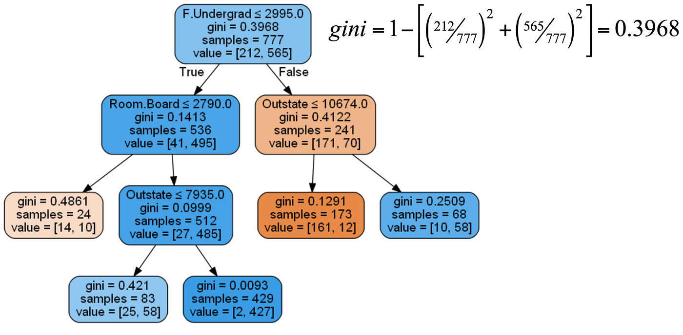
The ultimate goal of the decision tree algorithm is to create splits that result in pure leaf nodes—nodes that, ideally, contain samples from only one class. But how does the algorithm decide which questions to ask and in what order?

2. How a Decision Tree Learns: Finding the Best Split

The "magic" of a decision tree lies in how it chooses the best feature and the best value to split the data at each node. It does this by searching for the split that results in the "purest" possible child nodes. To quantify this purity, we use a metric. The two most common ones are Gini Impurity and Information Gain (based on Entropy).

We'll focus primarily on Gini Impurity, as it's the default criterion in scikit-learn and is very intuitive.

Gini Impurity

Gini Impurity measures the likelihood of incorrectly classifying a new instance from a dataset if it were randomly labeled according to the class distribution in that dataset.

• A Gini Impurity of 0 means a node is perfectly pure (all samples belong to one class).
• A Gini Impurity of 0.5 (for a binary classification problem) means a node is maximally impure (samples are split 50/50 between the two classes).

The formula for the Gini Impurity of a single node is:

where $C$ is the number of classes and $p_i$ is the proportion of samples belonging to class $i$ in that node.

To evaluate a split, the algorithm calculates a weighted average Gini Impurity of the child nodes. It chooses the split that yields the lowest weighted average Gini.

This might sound complex, but the StatQuest video makes it incredibly clear with a step-by-step example.

Information Gain (Alternative to Gini)

Another popular metric is Information Gain, which is based on a concept called Entropy. Like Gini Impurity, Entropy measures the level of disorder or impurity in a node. Information Gain calculates the reduction in entropy achieved by a split. The algorithm aims to find the split that provides the highest Information Gain.

3. Building the Tree: The Recursive Process

The algorithm builds the tree by applying this splitting logic recursively:

1. Start at the root node with the entire training dataset.
2. Find the best split: Test all features and all possible split points to find the one that minimizes the Gini Impurity (or maximizes Information Gain).
3. Split the data: Create two child nodes based on the best split.
4. Repeat: For each child node, repeat steps 2 and 3.
5. Stop: Continue this process until a stopping condition is met. This could be:
   • The node is perfectly pure.
   • The tree reaches a pre-defined maximum depth.
   • The number of samples in a node is too small to split further.

This recursive process is what creates the nested, tree-like structure.

4. Implementing a Decision Tree in Python

Now for the practical part. As usual, the scikit-learn library makes it incredibly simple to implement a decision tree. The process follows the familiar fit/predict pattern you saw with logistic regression.

The main class is DecisionTreeClassifier. Let's walk through an example.

Here's the core code from that tutorial, which you should recognize:

# 1. Import necessary libraries
from sklearn.tree import DecisionTreeClassifier
from sklearn.model_selection import train_test_split
from sklearn import metrics
import pandas as pd

# Assume 'pima' is a loaded Pandas DataFrame
# col_names = ['pregnant', 'glucose', 'bp', 'skin', 'insulin', 'bmi', 'pedigree', 'age', 'label']
# pima = pd.read_csv("diabetes.csv", header=None, names=col_names)
# pima = pima.iloc[1:] # remove header row if present

# 2. Select features and target
feature_cols = ['pregnant', 'insulin', 'bmi', 'age','glucose','bp','pedigree']
X = pima[feature_cols] # Features
y = pima.label # Target variable

# 3. Split data
X_train, X_test, y_train, y_test = train_test_split(X, y, test_size=0.3, random_state=1)

# 4. Create and train the model
# By default, this uses the 'gini' criterion
clf = DecisionTreeClassifier()
clf = clf.fit(X_train, y_train)

# 5. Make predictions
y_pred = clf.predict(X_test)

# 6. Evaluate the model
print("Accuracy:", metrics.accuracy_score(y_test, y_pred))

5. Preventing Overfitting: Pruning the Tree

If you let a decision tree grow to its full depth, it can become extremely complex and "memorize" the training data. This is called overfitting. An overfit model performs perfectly on the data it has seen but fails to generalize to new, unseen data.

To combat this, we can control the tree's complexity. One common method is pre-pruning, where we stop the tree from growing by setting limits. Two important hyperparameters for this are:

• max_depth: The maximum number of levels the tree can have.
• min_samples_leaf: The minimum number of samples required to be at a leaf node.

By tuning these parameters, you can create a simpler, more robust model.

By setting max_depth, we force the tree to stop splitting after a certain point, preventing it from learning noise in the training data. This is a crucial step in building practical machine learning models.

Conclusion

Congratulations! You have now learned about decision trees, a powerful and highly interpretable classification algorithm.

Key Takeaways:

• Decision trees create a model that predicts the value of a target variable by learning simple decision rules inferred from the data features.
• They are built by recursively splitting the data. At each node, the algorithm chooses the split that results in the purest child nodes.
• Gini Impurity and Information Gain are the two main metrics used to measure the quality of a split.
• The scikit-learn library provides the DecisionTreeClassifier class to easily build, train, and evaluate decision tree models.
• Uncontrolled trees can easily overfit. We can prevent this using pre-pruning techniques, such as setting the max_depth of the tree.

Preview of the Next Lesson:
We've now built a few classification models (Logistic Regression, k-NN, Decision Trees) and used "accuracy" as our primary evaluation metric. But is accuracy always the best measure of performance? What if one class is much rarer than another? In the first lesson of our next module, "Model Evaluation and Improvement," we will dive into a more sophisticated set of evaluation metrics, including precision, recall, and the F1-score, to get a more complete picture of a model's strengths and weaknesses.