Flatten vs. Ravel: View vs. Copy Behavior

1. From Many Dimensions to One

Often in data processing, you need to collapse a multi-dimensional tensor into a single, one-dimensional vector. For example, the output of a convolutional layer in an image recognition model is typically a multi-dimensional feature map, which must be flattened before being fed into a fully connected (dense) layer.

PyTorch, like NumPy, provides two main functions for this: flatten() and ravel(). At first glance, they appear to do the exact same thing.

import torch




# Create a 2x2x3 tensor
t = torch.arange(12).reshape(2, 2, 3)
print("Original tensor shape:", t.shape)



# Original tensor shape: torch.Size([2, 2, 3])




# Using flatten()
t_flat = t.flatten()
print("\nUsing flatten():")
print("Shape:", t_flat.shape)
print("Tensor:", t_flat)



# Shape: torch.Size([12])
# Tensor: tensor([ 0,  1,  2,  3,  4,  5,  6,  7,  8,  9, 10, 11])




# Using ravel()
t_ravel = t.ravel()
print("\nUsing ravel():")
print("Shape:", t_ravel.shape)
print("Tensor:", t_ravel)



# Shape: torch.Size([12])
# Tensor: tensor([ 0,  1,  2,  3,  4,  5,  6,  7,  8,  9, 10, 11])

As you can see, both methods successfully transformed the 3D tensor into a 1D tensor with 12 elements. So, why do both exist? The answer lies in how they handle the tensor's data in memory.

2. The Core Difference: View vs. Copy

The distinction between flatten() and ravel() is fundamental to memory management and performance, concepts you're well-acquainted with from software development. One operation creates a completely independent object in memory (a copy), while the other tries to provide a different look at the same underlying object (a view).

To see this in action, let's watch a short video. Although it uses NumPy, the principles and behavior of flatten and ravel are identical in PyTorch.

Let's confirm this behavior in PyTorch and introduce a useful function, shares_memory(), to programmatically check if two tensors share the same underlying data.

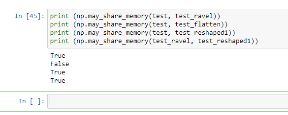
• tensor.flatten(): Always returns a new tensor, copying the data to a new location in memory. It is "safer" because it prevents unintentional changes to the original tensor.
• tensor.ravel(): Attempts to return a view of the original tensor, meaning it shares the same underlying data. This is more memory-efficient and faster as no data is copied.

Here's the code to prove it:

# Create a fresh tensor
t_original = torch.arange(6).reshape(2, 3)
print("Original tensor:\n", t_original)




# Test flatten()
t_flat = t_original.flatten()
print("\n--- Testing flatten() ---")
print("Shares memory with original:", t_original.shares_memory(t_flat)) # False



# Modify the flattened tensor
t_flat[0] = 99
print("Original tensor after modification:\n", t_original) # Unchanged




# ---




# Recreate the original tensor for a clean test
t_original = torch.arange(6).reshape(2, 3)




# Test ravel()
t_ravel = t_original.ravel()
print("\n--- Testing ravel() ---")
print("Shares memory with original:", t_original.shares_memory(t_ravel)) # True



# Modify the raveled tensor
t_ravel[0] = 99
print("Original tensor after modification:\n", t_original) # Changed!

This image, which uses the NumPy function np.may_share_memory (the equivalent of torch.shares_memory), provides a perfect visual summary of this behavior.

3. The ravel() Caveat: Contiguity Matters

You might have noticed I said ravel() attempts to return a view. When does it fail and resort to making a copy?

This brings us back to the concept of memory contiguity from our previous lessons. ravel() can only return a view if the tensor's data is laid out in a contiguous block of memory. If it's not, ravel() has no choice but to create a copy to produce a contiguous 1D array.

As we learned, operations like transpose(), permute(), or certain types of slicing can create non-contiguous tensors.

Let's read a quick explanation of this behavior.

Let's demonstrate this exact scenario in PyTorch, using transpose() to create a non-contiguous tensor.

# 1. Start with a contiguous tensor
t_cont = torch.arange(6).reshape(2, 3)
print("Is original tensor contiguous?", t_cont.is_contiguous()) # True




# Raveling it creates a view, as expected
t_cont_ravel = t_cont.ravel()
print("Raveled view shares memory:", t_cont.shares_memory(t_cont_ravel)) # True




# 2. Create a non-contiguous tensor via transpose
t_non_cont = t_cont.T  # .T is a shortcut for transpose(0, 1)
print("\nIs transposed tensor contiguous?", t_non_cont.is_contiguous()) # False




# 3. Ravel the non-contiguous tensor
t_non_cont_ravel = t_non_cont.ravel()



# Because the source is non-contiguous, ravel() must create a copy.
print("Raveled copy shares memory:", t_non_cont.shares_memory(t_non_cont_ravel)) # False




# Modifying the raveled tensor will NOT affect the transposed tensor
t_non_cont_ravel[0] = 999
print("\nOriginal transposed tensor after modification:\n", t_non_cont) # Unchanged

This behavior is crucial. If you're counting on ravel() to be a memory-saving view operation, you must be aware that previous operations on your tensor might silently force it to become a more expensive copy operation.

Finally, it's worth noting that reshape(-1) behaves identically to ravel(). It will also return a view if possible and a copy if not. However, using ravel() or flatten() makes your code more explicit about the intent to create a 1D tensor.

Conclusion

Congratulations on completing the first module! You've built a strong foundation for understanding how to manipulate tensor shapes and memory, a critical skill for any machine learning practitioner.

Key Takeaways:

• Both flatten() and ravel() collapse a multi-dimensional tensor into a 1D tensor.
• flatten() always returns a copy of the data. This is memory-intensive but prevents accidental modification of the original tensor.
• ravel() returns a view if the source tensor is contiguous, and a copy if it is not. This is generally more performant but requires you to be mindful of potential side effects on the original data.
• Your choice between them depends on your goal: use flatten() when you need a new, independent tensor, and ravel() when performance is key and you are either sure the data is contiguous or you don't mind potential side effects.

Preview of the Next Module:

We've spent this module focusing on the shape of a single tensor. In the next module, Broadcasting for Element-wise Operations, we'll dive into how PyTorch handles operations between tensors of different shapes. We'll start by exploring the purpose of broadcasting with a practical example, such as adding a vector of biases to a matrix of activations in a neural network.