Dijkstra's Algorithm for Shortest Paths

The Five Concepts for Today

We will build a deep, practical understanding of Dijkstra's algorithm through these five concepts:

1. The Core Problem: Defining the Single-Source Shortest Path (SSSP) problem.
2. The Greedy Approach & Relaxation: Understanding the core logic of greedily choosing the "closest" node.
3. The Algorithm Under the Hood: Using a Priority Queue for an efficient implementation.
4. Python Implementation & Complexity Analysis: Writing production-quality code and analyzing its performance.
5. The Critical Limitation & Interview Context: Why Dijkstra's fails with negative weights and how to discuss it in an interview.

Concept 1: The Core Problem - Single-Source Shortest Path

Technical Explanation

The Single-Source Shortest Path (SSSP) problem is defined as follows: given a weighted graph $G$, a source vertex $s$, find the path with the minimum total weight from $s$ to every other vertex $v$ in the graph. The "weight" of a path is the sum of the weights of the edges that constitute it.

Dijkstra's algorithm solves the SSSP problem for a crucial condition: all edge weights must be non-negative. This assumption is fundamental to the algorithm's correctness.

Real-world applications are everywhere:

• IP Routing: Finding the shortest path for data packets to travel through a network.
• GPS Navigation: Calculating the fastest route from your current location to a destination (where edge weights are travel times).
• Robotics/AI: Pathfinding for a robot in a physical space, minimizing distance or energy consumption.
• Social Networks: Finding the "closest" connection between two people (e.g., in LinkedIn's degree-of-separation feature).

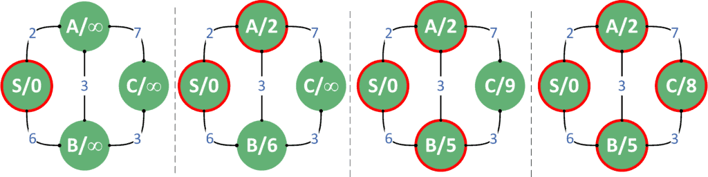
Metaphor: The GPS in Your Car

Imagine you're at home (the source node) and you want to know the fastest way to get to every other point of interest in your city. The roads are edges, and the time it takes to drive down a road is its weight.

Your GPS doesn't calculate all possible routes at once. It starts by saying, "The time to get home is 0." Then it looks at all roads connected directly to your home. It finds the closest intersection (A) and says, "The fastest way to get to A is X minutes." It then explores outward from A, always prioritizing the destination that is currently "fastest" to reach from your home. This greedy, expanding search is the essence of Dijkstra's algorithm.

Concept 2: The Greedy Approach & "Relaxation"

Technical Explanation

Dijkstra's is a greedy algorithm. At each step, it makes a locally optimal choice: it visits the unvisited vertex with the smallest known distance from the source. The "magic" of the algorithm lies in a process called relaxation.

Once we select the closest unvisited vertex, let's call it $u$, we explore its neighbors. For each neighbor $v$, we check if the path to $v$ through $u$ is shorter than any path to $v$ we've found so far.

This check is the relaxation step. Let dist[u] be the shortest distance from the source to $u$. The distance to a neighbor $v$ via $u$ would be dist[u] + weight(u, v). We compare this to the current best-known distance to v, dist[v].

The relaxation condition is:

If the condition is true, we have found a new, shorter path to $v$, so we update its distance.

To solidify this core concept, let's watch a video that explains relaxation very clearly.

Metaphor: Updating Your ETA

You're driving to a friend's house (V). Your GPS initially says the ETA is 30 minutes based on a known route. While you're driving, you pass a new junction (U) that you reached in 10 minutes. Your GPS realizes there's a side road from U to V that only takes 15 minutes.

It performs a "relaxation": the new time to V is (time to U) + (time from U to V) = 10 + 15 = 25 minutes. Since 25 is less than the old ETA of 30, it updates your route and ETA. You've "relaxed" the path to V by finding a better one.

Concept 3: The Algorithm Under the Hood (with a Priority Queue)

Technical Explanation

How do we efficiently find the unvisited vertex with the smallest distance at every step? A linear scan through all vertices would be slow, leading to an $O(V^2)$ algorithm. For sparse graphs, which are common in the real world, we can do much better.

The optimal solution uses a Min-Priority Queue (often implemented with a min-heap). This data structure is perfect for this task because it allows us to:

1. Store vertices, prioritized by their distance from the source.
2. Efficiently extract the vertex with the minimum distance in $O(\log V)$ time.

Here are the data structures we need:

• Adjacency List: A dictionary mapping each vertex to a list of its neighbors and the corresponding edge weights. E.g., graph = {u: [(v1, w1), (v2, w2), ...]}.
• Distances Map/Array: Stores the current shortest distance from the source to every other vertex. Initialized to $\infty$ for all nodes except the source, which is 0.
• Priority Queue (Min-Heap): Stores (distance, vertex) tuples. The heap property ensures the tuple with the smallest distance is always at the root, ready for extraction.

The Algorithm Flow:

1. Initialize distances with $\infty$ and distances[source] = 0.
2. Push (0, source) into the priority queue.
3. While the priority queue is not empty:
   a. Pop the element with the smallest distance: (d, u).
   b. If d > distances[u], it means we've found an even shorter path to u already. Skip this entry (this is a lazy update trick common with heaps).
   c. For each neighbor v of u with edge weight w:
   i. Relax the edge: If distances[u] + w < distances[v]:
   * Update distances[v] = distances[u] + w.
   * Push the new, better path info (distances[v], v) into the priority queue.
4. When the loop finishes, the distances map contains the shortest path lengths.

Concept 4: Python Implementation & Complexity Analysis

Technical Explanation

Let's translate the algorithm into clean, interview-ready Python code. We'll use Python's heapq module for the min-heap and a defaultdict for the adjacency list.

import heapq
from collections import defaultdict

def dijkstra(edges: list[list[int]], num_nodes: int, source: int):
    """
    Implements Dijkstra's algorithm to find the shortest path from a source
    to all other nodes in a weighted graph with non-negative weights.

    Args:
        edges: A list of edges, where each edge is [u, v, weight].
        num_nodes: The total number of nodes in the graph.
        source: The starting node.

    Returns:
        A dictionary mapping each node to its shortest distance from the source.
        Unreachable nodes will not be in the dictionary's keys.
    """
    # 1. Build adjacency list
    adj = defaultdict(list)
    for u, v, w in edges:
        adj[u].append((v, w))
    
    # 2. Initialize distances and priority queue
    shortest_paths = {} # Using a dict is flexible for disconnected graphs
    min_heap = [(0, source)] # (distance, node)

    # 3. Main loop
    while min_heap:
        # Get the node with the smallest distance so far
        dist, u = heapq.heappop(min_heap)

        # If we've already found a shorter path to u, skip
        if u in shortest_paths:
            continue
        
        # Lock in the shortest path to u
        shortest_paths[u] = dist

        # 4. Relaxation step
        for v, weight in adj[u]:
            if v not in shortest_paths:
                new_dist = dist + weight
                heapq.heappush(min_heap, (new_dist, v))
    
    # For a complete result as requested in many problems, fill in unreachable nodes
    for i in range(num_nodes):
        if i not in shortest_paths:
            shortest_paths[i] = -1 # Or float('inf') depending on problem spec

    return shortest_paths

# Example from a typical interview problem
num_nodes_ex = 6
edges_ex = [[0,1,2], [0,2,4], [1,2,1], [1,3,7], [2,4,3], [3,5,1], [4,3,2], [4,5,5]]
source_node = 0

print(f"Shortest paths from node {source_node}: {dijkstra(edges_ex, num_nodes_ex, source_node)}")
# Expected output for reachable nodes: {0: 0, 1: 2, 2: 3, 4: 6, 3: 8, 5: 9}

Complexity Analysis

Understanding the complexity is non-negotiable for top-tier interviews. Let $V$ be the number of vertices and $E$ be the number of edges.

• Time Complexity: $O(E\log V)$

  • Building the adjacency list: $O(E)$.
  • The while loop can run, in the worst case, until every vertex is processed. Extracting the minimum from the heap (heappop) takes $O(\log V)$ time. Since we do this for up to $V$ vertices, this part is $O(V\log V)$.
  • For every edge $(u,v)$, we might push a new distance to the heap (heappush). This happens at most $E$ times over the entire execution. Each push costs $O(\log V)$. This part is $O(E\log V)$.
  • Combining these, the total time complexity is $O(V\log V+E\log V)$. In a connected graph, $E\ge V-1$, so the $E\log V$ term dominates. Therefore, the complexity is $O(E\log V)$.

• Space Complexity: $O(V+E)$

  • Adjacency list: $O(V+E)$.
  • shortest_paths dictionary: $O(V)$.
  • Min-heap: In the worst case (a dense graph), the heap could hold an entry for many edges, but since we're pushing (distance, node) pairs, the number of distinct nodes in the heap is at most $V$. However, multiple paths to the same node can exist in the heap simultaneously in this lazy implementation. A dense graph could push $O(E)$ items. So, the heap could take up to $O(E)$ space.
  • Overall space is dominated by the adjacency list and the heap, resulting in $O(V+E)$.

Concept 5: The Critical Limitation & Interview Context

Technical Explanation

Dijkstra's algorithm only works if all edge weights are non-negative.

This is because of its greedy nature. When Dijkstra's finalizes the shortest path to a vertex u, it assumes it will never find a shorter path to u. A negative edge could violate this assumption. Imagine we finalize the path to u. Later, we explore a path to another vertex x that has a negative-weight edge leading back to a node on the path to u, creating a "cheaper" path to u after we've already locked it in. Dijkstra's never looks back, so it would miss this and produce an incorrect result.

Metaphor: The Irreversible Toll Road

Imagine our GPS system again. Once you pay a toll and pass a checkpoint (U), the system confirms your path and time. It will never consider routes that loop back to before that checkpoint, because that would always take more time... unless one of those loop-back roads was a "magic" road that paid you to drive on it (a negative weight). Dijkstra's algorithm assumes no such magic roads exist. Once a checkpoint is passed, it's considered done.

Conclusion

You have now mastered Dijkstra's algorithm, a titan of graph theory. You understand its greedy core, how to implement it efficiently with a priority queue, and, most importantly, its primary limitation.

Key Takeaways:

• Dijkstra's Algorithm solves the single-source shortest path problem in weighted graphs.
• It is a greedy algorithm that works by iteratively visiting the closest unvisited node and relaxing its neighbors.
• The crucial constraint is that all edge weights must be non-negative.
• The most efficient implementation uses an adjacency list and a min-priority queue (heap), yielding a time complexity of $O(E\log V)$.
• Failing to account for the non-negative weight constraint is a common interview pitfall.

Preview of the Next Lesson:
We've identified the Achilles' heel of Dijkstra's algorithm: negative edge weights. So, what do we do when our graph does have them? In our next lesson, we will cover the Bellman-Ford algorithm, a more robust (though slower) algorithm designed specifically to handle graphs with negative edge weights and to detect negative cycles.