Dynamic Array Implementation and Amortized Analysis

Concept 1: The Static Array's Limitation

To understand why dynamic arrays are necessary, we must first appreciate the rigid nature of their predecessor: the static array.

Technical Explanation

A traditional or "static" array is a contiguous block of memory of a fixed size. When you declare an array of size N, the system allocates a single, unbroken chunk of memory large enough to hold N elements of a specific type. This contiguity is the source of its greatest strength—fast, $O(1)$ access to any element via its index i (calculated as start_address + i * element_size)—and its greatest weakness. If you fill the array and need to add an (N+1)-th element, you can't. The memory adjacent to your array may already be in use. You are out of space.

Metaphor: The Egg Carton

Think of a static array as a standard one-dozen egg carton. It's designed to hold exactly 12 eggs. The positions are fixed, and you can instantly grab the 3rd egg or the 8th egg. However, if you come home with a 13th egg, you have a problem. You can't just tack on an extra slot to the carton. The carton is a fixed size. To store the 13th egg, you'd need a new, larger carton.

Python Code Snippet

While Python's built-in list is dynamic, we can simulate a fixed-size array using the ctypes module. This is closer to how arrays work in languages like C.

import ctypes

# Create a fixed-size array class (for demonstration)
class FixedArray:
    def __init__(self, size):
        self._size = size
        # Allocate a raw array of 'size' Python objects
        self._array = (size * ctypes.py_object)()
        for i in range(size):
            self._array[i] = None # Initialize with None
    
    def __setitem__(self, index, value):
        if not 0 <= index < self._size:
            raise IndexError("Index out of bounds")
        self._array[index] = value
        
    def __getitem__(self, index):
        if not 0 <= index < self._size:
            raise IndexError("Index out of bounds")
        return self._array[index]
        
    def __str__(self):
        return str([self._array[i] for i in range(self._size)])

# Let's try to use it
my_fixed_array = FixedArray(5)
my_fixed_array[0] = 10
my_fixed_array[4] = 50
print(f"Fixed array: {my_fixed_array}")

# Now, let's try to add a 6th element...
try:
    my_fixed_array[5] = 60 # This will fail
except IndexError as e:
    print(f"Error: {e}")

This demonstrates the core limitation we need to overcome.

Concept 2: The Core Mechanism of Resizing

The solution to the static array's limitation is conceptually simple: when you run out of space, you acquire a bigger space and move everything over.

Technical Explanation

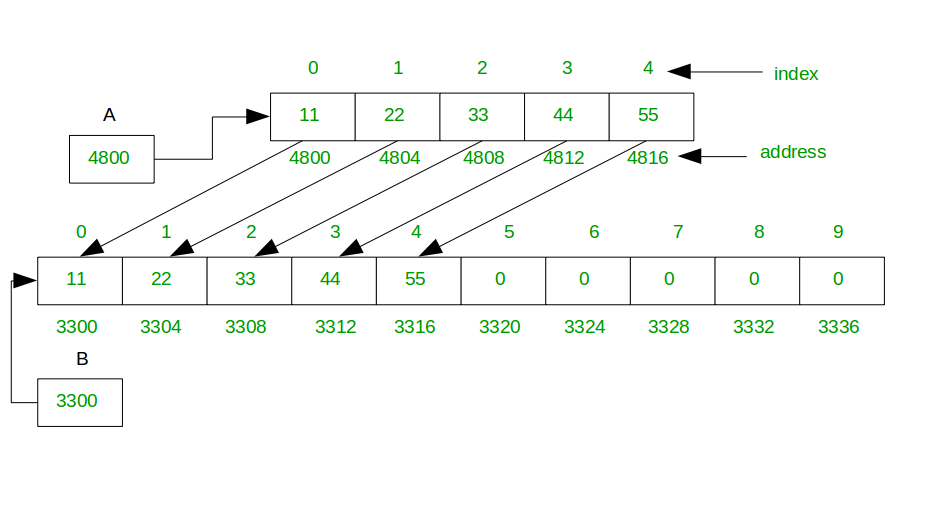
The resizing operation is the heart of a dynamic array. It involves three steps:

1. Allocate: Create a new, larger static array in memory.
2. Copy: Iterate through every element of the old, full array and copy it into the new, larger array.
3. Replace: Update the internal pointer of our data structure to refer to the new array. The old array is then deallocated (in memory-managed languages like Python, it is marked for garbage collection).

This copy operation is the expensive part. If we have N elements, it takes $O(N)$ time to copy them all to the new array.

Metaphor: Moving to a Bigger Apartment

Imagine your current apartment is full, and you acquire a new piece of furniture. You can't just knock down a wall to make more space. Instead, you have to:

1. Find and lease a new, bigger apartment (allocate).
2. Spend a whole day packing all your belongings and moving them to the new apartment (copy).
3. Update your mailing address and tell everyone your new location (replace).

The move itself is a lot of work ($O(N)$), but once you're done, you have plenty of room to add more things easily.

Python Code Snippet

Let's implement a private _resize method within a DynamicArray class. This function will be the workhorse for our automatic resizing.

import ctypes

class DynamicArray:
    def __init__(self):
        self._length = 0  # Number of actual elements
        self._capacity = 1  # Capacity of the underlying array
        self._array = self._make_array(self._capacity)

    def _make_array(self, capacity):
        # Helper to create a raw array
        return (capacity * ctypes.py_object)()

    def _resize(self, new_capacity):
        """Resize internal array to a new capacity."""
        print(f"Resizing from {self._capacity} to {new_capacity}...") # For demonstration
        
        # 1. Allocate a new, larger array
        new_array = self._make_array(new_capacity)
        
        # 2. Copy elements from the old array to the new one
        for i in range(self._length):
            new_array[i] = self._array[i]
            
        # 3. Replace the old array and update capacity
        self._array = new_array
        self._capacity = new_capacity
        
    def __len__(self):
        return self._length

    def __str__(self):
        return f"[{', '.join(str(self._array[i]) for i in range(self._length))}]"

# We'll add the `append` method in the next step.

This _resize method is the key piece of machinery. Now, we need to decide when and how to call it.

Concept 3: The Growth Strategy - Doubling Capacity

Calling _resize is expensive. We want to do it as infrequently as possible. A naive strategy of increasing capacity by one (_resize(self._capacity + 1)) each time we're full would be disastrously slow, as every single append would trigger an $O(N)$ copy operation. A much better approach is to grow the array exponentially.

Technical Explanation

The standard industry practice is to double the capacity of the array every time it becomes full. When length == capacity, we call _resize(2 * capacity). This means that after a resize, we have a large amount of "free" space, allowing for many subsequent append operations to be extremely fast $O(1)$ before the next expensive resize is needed. This trade-off—wasting some space to gain significant time efficiency—is central to system design.

To see this in action, let's watch a clear implementation walkthrough.

Metaphor: Buying a Bigger Bookshelf

Your bookshelf is full. You could buy a tiny shelf that holds just one more book. But then you'd be back at the store the next time you buy a book. This is like resizing by +1. A much smarter strategy is to buy a new bookshelf that's twice as big as your current one. It's a bigger upfront effort, but you won't have to think about buying another one for a long time. This is the doubling strategy.

Python Code Snippet

Let's add the append method to our DynamicArray class, incorporating the doubling strategy.

# (Continuing the DynamicArray class from above)

class DynamicArray:
    # ... (init, _make_array, _resize, __len__, __str__ from before) ...
    def __init__(self):
        self._length = 0
        self._capacity = 1
        self._array = self._make_array(self._capacity)

    def _make_array(self, capacity):
        return (capacity * ctypes.py_object)()

    def _resize(self, new_capacity):
        #print(f"Resizing from {self._capacity} to {new_capacity}...")
        new_array = self._make_array(new_capacity)
        for i in range(self._length):
            new_array[i] = self._array[i]
        self._array = new_array
        self._capacity = new_capacity
        
    def __len__(self):
        return self._length

    def __str__(self):
        items = [str(self[i]) for i in range(self._length)]
        return f"[{', '.join(items)}] (Length: {self._length}, Capacity: {self._capacity})"

    def __getitem__(self, k):
        if not 0 <= k < self._length:
            raise IndexError('invalid index')
        return self._array[k]

    def append(self, obj):
        """Add an object to the end of the array."""
        if self._length == self._capacity:
            # Double the capacity if the array is full
            self._resize(2 * self._capacity)
        
        # Add the new object and increment the length
        self._array[self._length] = obj
        self._length += 1

# Let's test it out
arr = DynamicArray()
for i in range(10):
    print(f"Appending {i}...")
    arr.append(i)
    print(f"Array state: {arr}")
    print("-" * 20)

Run this code and watch how the capacity grows exponentially: 1, 2, 4, 8, 16...

Concept 4: Worst-Case vs. Amortized Analysis

Now for the critical question: What is the time complexity of our append operation? The answer is "it depends." Most of the time it's $O(1)$, but occasionally it's a very slow $O(N)$. This is where amortized analysis becomes essential.

Technical Explanation

• Worst-Case Complexity: The worst possible time an operation can take. For append, this occurs when we trigger a resize. The cost is $O(N)$ to copy N elements.
• Average-Case Complexity: The expected time an operation takes, averaged over all possible inputs. This involves probability and isn't what we're doing here.
• Amortized Complexity: The worst-case average time an operation takes over a sequence of operations. It's a way to analyze algorithms where expensive operations are rare, and cheap operations are common. It guarantees the average performance of each operation in the sequence will be low, even if a single operation is occasionally expensive.

Metaphor: Daily Commute with Occasional Traffic Jams

Your daily commute to work usually takes 15 minutes ($O(1)$). However, once every few months, a major accident causes a massive traffic jam, and the commute takes 2 hours ($O(N)$).

If someone asks for the worst-case time, you'd have to say 2 hours. But this is misleading; it doesn't represent your typical experience. If you average your commute time over a whole year (a sequence of commutes), the average time is probably closer to 16 or 17 minutes. This average time, which smooths out the rare, expensive events, is the amortized time.

Concept 5: Proving O(1) Amortized Cost

We can mathematically prove that the amortized cost of append is $O(1)$. We will use two related methods: the Aggregate Method for a formal proof and the Banker's Method for a more intuitive understanding.

Technical Explanation: The Aggregate Method

This method calculates the total cost of a sequence of m operations and then divides by m to find the amortized cost.

Let's analyze a sequence of m appends to an empty array.

1. Cost of insertions: Each of the m appends has a base cost of 1 for inserting the element itself. Total cost = $m$.
2. Cost of resizing: Resizing happens when the number of elements k is a power of 2 (1, 2, 4, 8, ...). A resize at size k costs k to copy the k elements. The total cost of all resizes for m appends is the sum of these costs: $1+2+4+8+...+2^j$, where $2^j$ is the largest power of 2 less than or equal to m. This is a geometric series.

The total cost $C_{total}$ of m operations is:
$C_{total}=\underset{\text{insertions}}{\underbrace{m}}+\underset{\text{resizings}}{\underbrace{\sum _{j=0}^{\lfloor {\log }_2(m-1)\rfloor }{2}^j}}$
The sum of the geometric series ${\sum }_{j=0}^k{2}^j=2^{k+1}-1$. In our case, this sum is less than $2m$.
So, $C_{total}<m+2m=3m$.

The amortized cost per operation is $C_{total}/m<3m/m=3$.
Since the amortized cost is a constant (3), we say it is $O(1)$.

Intuitive Explanation: The Banker's Method

Imagine each append operation costs $3 (the amortized cost).

• $1 is used to pay for the actual insertion of the element.
• $2 are saved as "credits" and stored with the newly added element.

Now, consider what happens when the array is full and needs to resize from size k to 2k. At this moment, the array contains k elements. The most recent k/2 elements were added since the last resize. Each of these k/2 elements has $2 in credits saved up.
Total saved credits = $(k/2)\text{ elements}\times \$2/\text{element}=\$k$.

The cost of resizing is copying k elements, which costs exactly $k. We can pay for this entire expensive operation using our saved credits! The amortized cost of the resize itself becomes $0. Since every operation's amortized cost is constant ($3), the overall amortized cost is $O(1)$.

Conclusion

Today, you went "under the hood" of one of the most common data structures. You built a dynamic array from first principles, understanding not just what it does, but how it achieves its remarkable efficiency.

Key Takeaways:

• Static vs. Dynamic: Dynamic arrays overcome the fixed-size limitation of static arrays by intelligently resizing a backing static array.
• The Resize Mechanism: The core of a dynamic array is the process of allocating a larger array and copying over the existing elements, an $O(N)$ operation.
• Exponential Growth: Doubling the capacity on each resize is a crucial strategy that minimizes the frequency of expensive copy operations.
• Amortized Analysis: This is the correct tool for analyzing algorithms with occasional expensive operations. It provides a worst-case guarantee on the average cost per operation over a sequence.
• $O(1)$ Append Cost: Through both formal proof (Aggregate Method) and intuition (Banker's Method), you've shown that the append operation on a doubling dynamic array has an amortized time complexity of $O(1)$.

Preview of the Next Lesson

While dynamic arrays give us $O(1)$ amortized appends and $O(1)$ random access (__getitem__), they have weaknesses. Inserting or deleting an element at the beginning or in the middle requires shifting all subsequent elements, a slow $O(N)$ operation.

In our next lesson, we will explore a completely different approach to storing a list of items: singly and doubly linked lists. We will see how they excel where dynamic arrays are weak, and vice versa, setting up one of the most fundamental trade-off discussions in data structures.