Data and Model Parallelism

1. The 'Why': The Unavoidable Challenge of Scale (Easy)

• Technical Explanation:
  Modern deep learning models, especially Large Language Models (LLMs) and Vision Transformers, have grown to immense sizes. A model like GPT-3 has 175 billion parameters. Storing these parameters, along with their gradients and optimizer states (which are needed for training), requires hundreds of gigabytes of memory.

  This creates two fundamental bottlenecks:

  1. The Memory Wall: The largest available GPUs (like the NVIDIA A100 or H100) have around 80 GB of VRAM. A multi-billion parameter model simply cannot fit into the memory of a single device. The model's parameters, gradients, optimizer states, and the intermediate activations from the forward pass collectively exceed this limit.
  2. The Time Wall: Even if a model could fit, the sheer number of computations ($\text{petaflops}$) required to train it on a massive dataset would be prohibitive. A single GPU would take centuries to complete the task.

  Distributed training is not an optimization; it is a necessity to overcome these physical walls.

• Metaphor for a 5-Year-Old:
  Imagine you want to build a giant Lego castle that has a billion bricks (the model). First, you discover the instruction book and all the bricks won't even fit in your bedroom (the GPU's memory). That's the Memory Wall. Second, even if they did fit, you realize it would take you 100 years to build it by yourself. That's the Time Wall. The only solution is to get a team of friends and a bigger space to build it together.

• Real-World Anchor:
  To grasp the scale we're talking about, let's watch a short segment from a Stanford MLSys seminar.

2. Data Parallelism: The "Divide the Data" Strategy (Easy)

• Technical Explanation:
  Data parallelism is the most common and intuitive form of distributed training. It's used when the model can fit on a single GPU, but you want to accelerate training by processing more data in parallel.

  The process, often implemented using PyTorch's DistributedDataParallel (DDP), follows these steps:

  1. Replicate: The entire model is copied onto each of the $N$ available GPUs (workers).
  2. Shard: The global batch of training data is split into $N$ smaller mini-batches. Each worker receives its own unique mini-batch.
  3. Compute: Each worker independently performs a forward and backward pass on its mini-batch to compute its local gradients. At this point, each worker has a different set of gradients because they saw different data.
  4. Synchronize: The gradients from all workers are aggregated into a single, averaged gradient. This is achieved using a highly efficient collective communication operation called All-Reduce. After this step, every worker has the exact same, final gradient.
  5. Update: Each worker uses the synchronized gradient to update its local copy of the model weights. Because they all start with the same weights and apply the same update, their models remain identical.

*This image illustrates two ways to average gradients. The Parameter Server was an early model. Modern systems like PyTorch's DDP use a decentralized Peer-to-Peer approach like **Ring All-reduce**, which is more efficient and avoids a central bottleneck.*

• Metaphor for a 5-Year-Old:
  A team of four chefs (workers) are trying to perfect a new cake recipe (the model). They all start with the exact same recipe book.

  1. Each chef gets a different bag of ingredients (a mini-batch of data).
  2. They each bake their own cake and take notes on how to improve the recipe (local gradients). Chef 1 thinks it needs more sugar; Chef 2 thinks it needs less flour.
  3. They all get on a conference call (All-Reduce) and average their suggestions to agree on one single change.
  4. Each chef then makes that same change in their own recipe book. Now they all have the same, slightly improved recipe for the next round of baking.

• Python Code Snippet (Conceptual DDP):
  This is what the setup looks like in PyTorch. The key is wrapping your model with DistributedDataParallel. The library handles the gradient synchronization under the hood.

```python
import torch
import torch.nn as nn
from torch.utils.data.distributed import DistributedSampler
from torch.nn.parallel import DistributedDataParallel as DDP
import torch.distributed as dist
import os

def setup(rank, world_size):
    """Initializes the distributed environment."""
    os.environ['MASTER_ADDR'] = 'localhost'
    os.environ['MASTER_PORT'] = '12355'
    dist.init_process_group("gloo", rank=rank, world_size=world_size)

# --- On each worker process ---
# rank = # current process id
# world_size = # total number of processes

# 1. Setup the process group
# setup(rank, world_size)

# 2. Create the model and move it to the correct device
model = nn.Linear(10, 10).to(rank)
# 3. Wrap the model with DDP
ddp_model = DDP(model, device_ids=[rank])

# 4. Create a DistributedSampler to shard the data
# sampler = DistributedSampler(dataset, num_replicas=world_size, rank=rank)
# dataloader = DataLoader(dataset, sampler=sampler)

# --- Training loop ---
# for data, labels in dataloader:
#     optimizer.zero_grad()
#     outputs = ddp_model(data.to(rank))
#     loss = loss_fn(outputs, labels.to(rank))
#     loss.backward()  # DDP automatically synchronizes gradients here
#     optimizer.step()

# dist.destroy_process_group()
```

3. Model Parallelism: The "Divide the Model" Strategy (Medium)

• Technical Explanation:
  Model parallelism tackles the Memory Wall. When a model is too large to fit on a single GPU, you have no choice but to partition the model itself across multiple devices.

  In its simplest form (inter-layer parallelism), the layers of the model are split sequentially across GPUs.

  • GPU 0 might hold layers 1-16.
  • GPU 1 might hold layers 17-32.
  • and so on.

  During a forward pass, the input data is processed by GPU 0, and its output activations are sent to GPU 1. GPU 1 then performs its computation and passes the result to the next GPU in the chain. The backward pass works in reverse, with gradients flowing backward through the GPUs. This introduces a significant communication cost at the boundary of each GPU partition.

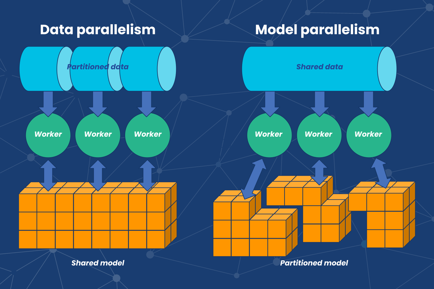
This diagram provides a clear contrast. In Data Parallelism (left), the model is replicated, and the data is split. In Model Parallelism (right), the data is replicated (or passed along), and the model is split.

• Metaphor for a 5-Year-Old:
  Your Lego castle is now so gigantic it requires four different rooms (GPUs) to build.

  • Your friends in Room 1 build the foundation (layers 1-16).
  • They pass the partially built structure through a hallway (the network) to Room 2.
  • The team in Room 2 adds the castle walls (layers 17-32).
  • They pass it to Room 3, where another team adds the towers.
    This continues until the castle is complete. Unlike the data parallelism chefs who all worked at the same time, this is an assembly line where each team must wait for the previous one to finish.

• Reading:
  For a formal definition, you can refer to the following academic survey.

4. Under the Hood: Flavors of Model Parallelism (Hard)

• Technical Explanation:
  "Model Parallelism" is an umbrella term. In practice, two sophisticated forms are used to train SOTA models, often in combination:

  A) Tensor Parallelism (Intra-layer):
  Instead of splitting between layers, tensor parallelism splits the large weight matrices within a single layer (like a Transformer's self-attention or MLP block) across multiple GPUs. For example, a matrix multiplication $Y=XA$ can be parallelized by splitting the matrix $A$ column-wise across two GPUs: $A=[A_1,A_2]$. Each GPU computes part of the result ($X{A}_1$ and $X{A}_2$), and the results are gathered. This requires high-speed, low-latency communication (e.g., NVIDIA's NVLink) and is most effective within a single server node.

  B) Pipeline Parallelism (Inter-layer):
  This is the assembly line we described earlier. It partitions sequential blocks of layers across different GPUs/nodes. The major challenge is the "pipeline bubble"—the idle time at the start and end of a batch where GPUs are waiting for work. To mitigate this, the training batch is split into smaller micro-batches, which are fed into the pipeline one after another, allowing GPUs to work in parallel on different micro-batches. Even with this optimization, some idle time is unavoidable.

• Metaphor for a 5-Year-Old:
  Back to our assembly line for the giant Lego castle:

  • Pipeline Parallelism: This is the assembly line itself. Room 1 does foundations, Room 2 does walls.
  • Tensor Parallelism: Inside Room 1, the foundation is so complex that four people work on it at the same time. One lays the left-front corner, another the right-front, etc. They are all working on the same step (the foundation layer), just different parts of it.

• Deep Dive Video:
  The Stanford seminar provides the best visual explanation of these concepts.

5. The Synthesis: Combining Parallelism Strategies (Harder)

• Technical Explanation:
  No single parallelism strategy is sufficient for training trillion-parameter models. Elite systems at Google, Meta, and NVIDIA use a hybrid approach that combines all three. A common configuration for a large cluster of GPUs might be:

  1. Tensor Parallelism: Used within each server node to split the model's individual layers across the 8 GPUs connected by high-speed NVLink. Let's say tensor_model_parallel_size = 8.
  2. Pipeline Parallelism: Used across different server nodes to partition the entire sequence of model layers. If the model is split into 16 pipeline stages, pipeline_model_parallel_size = 16.
  3. Data Parallelism: The remaining available GPUs are used for data parallelism. Each "model replica" (which is itself a pipeline of tensor-parallel groups) gets a different shard of the data. The data_parallel_size is calculated from the total number of GPUs.

  If you have a total of 1024 GPUs:

  $$\text{world\_size}=\text{DP\_size}\times \text{PP\_size}\times \text{TP\_size}$$ $$1024=\text{DP\_size}\times 16\times 8⟹\text{DP\_size}=\frac{1024}{128}=8$$

  This means you'd have 8 full model replicas, each training on a different part of the data.

• Metaphor for a 5-Year-Old:
  We need to build a whole fleet of 8 identical, giant Lego castles (Data Parallelism).

  • For each castle, we set up a 16-room assembly line (Pipeline Parallelism).
  • Inside each of the 16 rooms, an 8-person team works together on their specific section (Tensor Parallelism).
  • All 8 castle factories run simultaneously, allowing us to build the entire fleet much faster.

• Practical Example & Trade-offs:
  This combination isn't arbitrary; it's about optimizing communication. Tensor parallelism requires the fastest interconnect, so it's kept within a node. Pipeline parallelism can tolerate the slightly higher latency between nodes. Data parallelism has the least frequent communication (one All-Reduce per step), making it suitable for the highest scale.

This configuration is exactly what's done in frameworks like NVIDIA's Megatron-LM.

Conclusion

Today, you've learned the fundamental strategies that make training today's enormous AI models possible. This is a critical concept that separates standard ML practitioners from engineers who can build and operate systems at massive scale.

Key Takeaways:

• Distributed training is necessary to overcome the memory and time walls of modern deep learning.
• Data Parallelism scales training by replicating the model and sharding the data. It's ideal when the model fits on one GPU.
• Model Parallelism scales the model size by partitioning the model itself across multiple GPUs.
• The two key types of model parallelism are Tensor Parallelism (intra-layer, for fast interconnects) and Pipeline Parallelism (inter-layer, for scaling across nodes).
• State-of-the-art systems use a hybrid strategy, combining all three types of parallelism to balance memory constraints, compute efficiency, and communication overhead.

Next Lesson Preview

We now understand how to distribute the computational work of training. But in a production environment, how do we manage the data that feeds these models in a scalable, reusable, and consistent way? Our next lesson will introduce the architecture of a feature store, a critical MLOps component for managing ML features and preventing the dreaded problem of training-serving skew.