AVL Tree Rotations for Self-Balancing BSTs

Concept 1: The "Why" - The Peril of Unbalanced Trees

First, let's solidify why we need self-balancing trees at all. While a perfectly balanced BST offers $O(\log N)$ performance, this is only the average or best case. The worst case is a critical vulnerability in any production system.

Technical Explanation

A Binary Search Tree's structure is entirely dependent on the order of insertion. If we insert keys in a sorted or nearly-sorted order (e.g., 1, 2, 3, 4, 5, 6, 7), the tree becomes "skewed" or "degenerate." It effectively turns into a linked list.

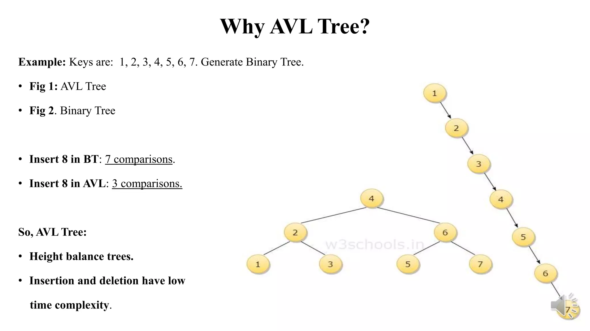
A self-balancing BST, like an AVL tree, is a BST that automatically performs structural modifications—called rotations—after insertions or deletions to ensure the tree remains "shallow" or "bushy." This guarantees that its height stays close to the optimal ${\log }_2(N)$, ensuring all core operations remain at a worst-case time complexity of $O(\log N)$.

Metaphor: The Unorganized vs. The Self-Organizing Library

Imagine a library where new books are always placed on the next available shelf space, moving from left to right. If a large shipment of books all starting with 'A' arrives, they will fill up all the shelves on the left side of the library. To find a book starting with 'B', you'd have to walk past this entire massive 'A' section. This is an unbalanced BST.

Now, imagine a self-organizing library. When the new 'A' books arrive, the librarian doesn't just put them on the shelves. They notice one section is getting too full and rearrange the shelves themselves—moving entire aisles—to keep the overall layout balanced. Finding any book remains quick because the library's structure is always maintained. This is a self-balancing tree.

Concept 2: The AVL Invariant - The Balance Factor

How does an AVL tree know when it's time to "reorganize the shelves"? It uses a strict rule called the AVL-tree property, which is enforced using a metric called the balance factor.

Technical Explanation

For every single node in an AVL tree, the heights of its left and right subtrees can differ by at most 1. The balance factor (BF) of a node is formally defined as:

By convention:

• The height of a None or null node is -1.
• The height of a leaf node is 0.
• The height of any other node is 1 + max(height(left_child), height(right_child)).

For a tree to be a valid AVL tree, the balance factor of every node must be in the set $\{-1,0,1\}$.

• BF = 1: The node is "left-heavy."
• BF = -1: The node is "right-heavy."
• BF = 0: The node is perfectly balanced.

If an insertion or deletion causes any node's balance factor to become 2 or -2, the tree is considered unbalanced, and a rotation is triggered to restore the property.

To dive deeper into this core concept, watch the following video segment.

Metaphor: The Tightrope Walker

Think of each node in the tree as a tightrope walker. Their left arm represents the left subtree, and their right arm the right subtree. They can stay balanced by keeping their arms at roughly the same level.

• Slightly leaning left (left arm lower) is a balance factor of 1.
• Slightly leaning right (right arm lower) is a balance factor of -1.
• Arms perfectly level is a balance factor of 0.

If they lean too far in one direction (a balance factor of 2 or -2), they are about to fall. Before they do, they must perform a quick, corrective hop (a rotation) to regain their balance.

Concept 3: Simple Rebalancing - Single Rotations

When a tree becomes unbalanced in a "straight line," we can fix it with a single, elegant maneuver: a single rotation. There are two symmetric cases: Left-Left and Right-Right.

Technical Explanation

Let's say z is the first unbalanced node (BF=2 or -2) we find when moving up from the inserted node.

1. Left-Left Case (BF of z is 2, BF of z.left is 1): This means z is left-heavy, and its left child is also left-heavy. The imbalance is caused by an insertion into the left subtree of the left child of z.

   • Solution: Perform a Right Rotation on z.
   • Mechanics: The left child of z (let's call it y) moves up to take z's place. z becomes the right child of y. The original right child of y becomes the new left child of z. This maintains the BST property while rebalancing the heights.

2. Right-Right Case (BF of z is -2, BF of z.right is -1): This is the mirror image. z is right-heavy, and its right child is also right-heavy. The imbalance is in the right subtree of the right child of z.

   • Solution: Perform a Left Rotation on z.
   • Mechanics: The right child y moves up. z becomes the left child of y. The original left child of y becomes the new right child of z.

Metaphor: Re-hooking a Mobile Sculpture

Imagine a hanging mobile sculpture with three main pieces in a line: A, B, and C, where A is above B, and B is above C (a Left-Left imbalance). The whole thing is tilting heavily to one side. To fix it, you don't add weight; you re-hook the structure. You unhook B from A, and re-hook A underneath B on the other side. Now, B is at the top, with A and C hanging balanced beneath it. You've performed a right rotation.

Concept 4: Complex Rebalancing - Double Rotations

What if the imbalance isn't a straight line but has a "kink" or "dogleg"? This happens in the Left-Right and Right-Left cases, and requires a double rotation.

Technical Explanation

Again, let z be the unbalanced node.

1. Left-Right Case (BF of z is 2, BF of z.left is -1): z is left-heavy, but its left child y is right-heavy. The imbalance is caused by an insertion into the right subtree of the left child of z.

   • Solution: A single rotation won't work. We first need to "straighten the kink."
     1. Perform a Left Rotation on the child, y. This transforms the subtree into a standard Left-Left case.
     2. Now, perform a Right Rotation on the original unbalanced node, z.

2. Right-Left Case (BF of z is -2, BF of z.right is 1): The mirror image. z is right-heavy, but its right child y is left-heavy.

   • Solution:
     1. Perform a Right Rotation on the child, y, to transform it into a Right-Right case.
     2. Perform a Left Rotation on z.

This image provides a perfect summary of all four rotation cases.

Metaphor: Fixing a Bent Chain Link

Imagine a chain hanging from z, with a link y below it, but the next link x is bent sideways (a Left-Right case). You can't just pull on z to straighten the whole chain; it'll just stay bent.

1. First, you must grab link y and twist it, which brings x into a straight line below y. This is the first rotation (a left rotation on y).
2. Now the whole chain is hanging in a straight, but still too long, line (z-x-y). This is a simple Left-Left case. A single pull (a right rotation on z) will now balance the entire structure.

Concept 5: The Full Picture - AVL Insertion and Trade-offs

Now let's assemble these pieces into a complete algorithm for insertion and discuss the architectural implications—a key focus for elite engineering roles.

Technical Explanation: The insert Algorithm

1. Standard BST Insert: First, insert the new node just as you would in a regular BST.
2. Walk and Update: Traverse back up the tree from the new node's parent to the root. In this post-insertion path:
   a. Update Height: Recalculate and update the height of each ancestor node.
   b. Check Balance Factor: Calculate the balance factor of the current ancestor.
   c. Rebalance if Needed: If the balance factor is 2 or -2, you've found the unbalanced node z.
   i. Identify which of the four cases (LL, RR, LR, RL) you have by checking the balance factor of z's child (y) on the insertion path.
   ii. Perform the corresponding single or double rotation.
   d. Stop: For an insertion, once you perform a single rebalancing operation, the heights of the subtree are restored to what they were before the insertion. You do not need to continue checking up the tree.

Python Code Snippet: AVL Insertion

Here is a recursive implementation that cleanly shows the rebalancing logic.

class AVLNode:
    def __init__(self, key):
        self.key = key
        self.left = None
        self.right = None
        self.height = 0 # Height of a new node is 0

class AVLTree:
    def get_height(self, node):
        return node.height if node else -1

    def get_balance(self, node):
        return self.get_height(node.left) - self.get_height(node.right) if node else 0

    def _right_rotate(self, z):
        y = z.left
        T3 = y.right
        # Perform rotation
        y.right = z
        z.left = T3
        # Update heights
        z.height = 1 + max(self.get_height(z.left), self.get_height(z.right))
        y.height = 1 + max(self.get_height(y.left), self.get_height(y.right))
        return y

    def _left_rotate(self, z):
        y = z.right
        T2 = y.left
        # Perform rotation
        y.left = z
        z.right = T2
        # Update heights
        z.height = 1 + max(self.get_height(z.left), self.get_height(z.right))
        y.height = 1 + max(self.get_height(y.left), self.get_height(y.right))
        return y

    def insert(self, root, key):
        # 1. Standard BST insertion
        if not root:
            return AVLNode(key)
        elif key < root.key:
            root.left = self.insert(root.left, key)
        else:
            root.right = self.insert(root.right, key)

        # 2. Update height of this ancestor node
        root.height = 1 + max(self.get_height(root.left), self.get_height(root.right))

        # 3. Get the balance factor
        balance = self.get_balance(root)

        # 4. If unbalanced, perform rotations
        # Left-Left Case
        if balance > 1 and key < root.left.key:
            return self._right_rotate(root)

        # Right-Right Case
        if balance < -1 and key > root.right.key:
            return self._left_rotate(root)

        # Left-Right Case
        if balance > 1 and key > root.left.key:
            root.left = self._left_rotate(root.left)
            return self._right_rotate(root)

        # Right-Left Case
        if balance < -1 and key < root.right.key:
            root.right = self._right_rotate(root.right)
            return self._left_rotate(root)

        return root

Real-World System Trade-offs: AVL vs. Red-Black Tree

In a system design interview, you won't just be asked to implement an AVL tree, but to justify why you'd choose it over another self-balancing tree, like a Red-Black Tree.

• AVL Trees are more strictly balanced. Their height is guaranteed to be at most $\approx 1.44{\log }_{2}N$. This makes them slightly faster for lookups (reads) because the tree is guaranteed to be shallower.
• Red-Black Trees are more relaxed. Their height can be up to $2{\log }_{2}N$. This means they require fewer and simpler rotations on average to maintain balance during insertions and deletions. This makes them faster for write-heavy workloads.
• Industry Use Cases:
  • AVL Trees are excellent for lookup-intensive applications, like a dataset that is built once and searched many times (e.g., language dictionaries, object sets in CAD software).
  • Red-Black Trees are more common in general-purpose applications with a mix of reads and writes. This is why they are used to implement std::map in C++ and TreeMap in Java. They are also used extensively in OS process schedulers.

Conclusion

You have now mastered the core principles of self-balancing trees, a critical concept for robust software engineering. You've seen that the perceived complexity of AVL trees boils down to a simple rule (the balance factor) and a set of four mechanical responses (the rotations).

Key Takeaways:

• Problem: Standard BSTs can become skewed, leading to $O(N)$ worst-case performance. Self-balancing trees guarantee $O(\log N)$ performance.
• AVL Property: The height difference between the left and right subtrees of any node (the balance factor) must not exceed 1.
• Rotations: Four types of imbalances (Left-Left, Right-Right, Left-Right, Right-Left) are fixed by two types of single rotations (Left, Right) and two types of double rotations (Left-Right, Right-Left).
• Insertion Algorithm: After a standard BST insert, walk back up the tree, updating heights and performing a single rebalancing operation at the first unbalanced node found.
• Architectural Choice: AVL trees are stricter and thus faster for read-heavy workloads, while Red-Black trees are more common in general-purpose libraries due to faster average write performance.

Preview of the Next Lesson

We are now concluding our deep dive into hierarchical data structures and will pivot to Module 4: Hashing, Sets, and Range Queries. Our first lesson will be foundational: you will implement a hash table using both chaining and open addressing for collision resolution. This is arguably the most important data structure in all of computer science, and understanding its "under the hood" mechanics is essential for any elite engineer.