LSM Trees: Architecture & Read/Write Trade-offs

1. The Write Bottleneck: Why B-Trees Aren't Always the Answer (Easy)

• Technical Explanation:
  Most traditional relational databases (like PostgreSQL, MySQL) use a data structure called a B-Tree to store data on disk. A B-Tree is a self-balancing tree that keeps data sorted, which makes it incredibly efficient for reads. To find a piece of data, you traverse the tree from the root to a leaf node in logarithmic time, which typically involves just a few disk seeks.

  However, B-Trees perform in-place updates. When you write or update a record, the database must find the correct page on disk, load it into memory, modify it, and write it back. If the page is full, it might need to be split, causing a cascade of updates to parent nodes. This process involves multiple random I/O operations, which are notoriously slow on both spinning hard drives and even modern SSDs. For write-heavy workloads (e.g., ingesting logs, metrics, or user events), this random write pattern becomes a major performance bottleneck.

• Metaphor for a 5-Year-Old:
  Imagine a B-Tree is a perfectly organized, alphabetized bookshelf.

  • Reading: Finding a book is super fast. If you want the book "Dune", you go straight to the 'D' section.
  • Writing: Adding a new book, "Dune Messiah," is slow. You have to go to the 'D' section, find the exact spot between "Dune" and "Dunkirk", and carefully shift all the other books to make space. If the shelf is full, you have to move books to another shelf and update your directory. It's a lot of work for one new book.

• Python Code Snippet (Conceptual):
  We won't implement a B-Tree, but this conceptual snippet highlights the logic of an in-place update versus an append-only one.

  # Represents a page on disk in a B-Tree like structure
  # Updates happen 'in-place'
  data_page = {'user:100': '{"name": "Alice"}', 'user:102': '{"name": "Charlie"}'}
  
  def b_tree_style_update(page, key, value):
      print(f"Executing B-Tree style update for key: {key}")
      # 1. Find the right page (we assume we have it)
      # 2. Modify the data directly in the page
      print("  - Performing random I/O to update data in-place...")
      page[key] = value
      print("  - Update complete.")
      return page
  
  # Represents an append-only log
  # New data is just added to the end
  log = ['{"key": "user:100", "value": "Alice"}', '{"key": "user:102", "value": "Charlie"}']
  
  def log_style_write(log_file, key, value):
      print(f"Executing Log style write for key: {key}")
      # 1. Just append the new data to the end of the file
      print("  - Performing sequential I/O to append data...")
      log_file.append(f'{{"key": "{key}", "value": "{value}"}}')
      print("  - Append complete.")
      return log_file
  
  print("--- B-Tree Scenario ---")
  data_page = b_tree_style_update(data_page, 'user:101', '{"name": "Bob"}')
  print(f"Final Page State: {data_page}\n")
  
  print("--- Log-based Scenario ---")
  log = log_style_write(log, 'user:101', '{"name": "Bob"}')
  print(f"Final Log State: {log}")
  

2. The LSM-Tree Write Path: The Beauty of Sequential Appends (Medium)

• Technical Explanation:
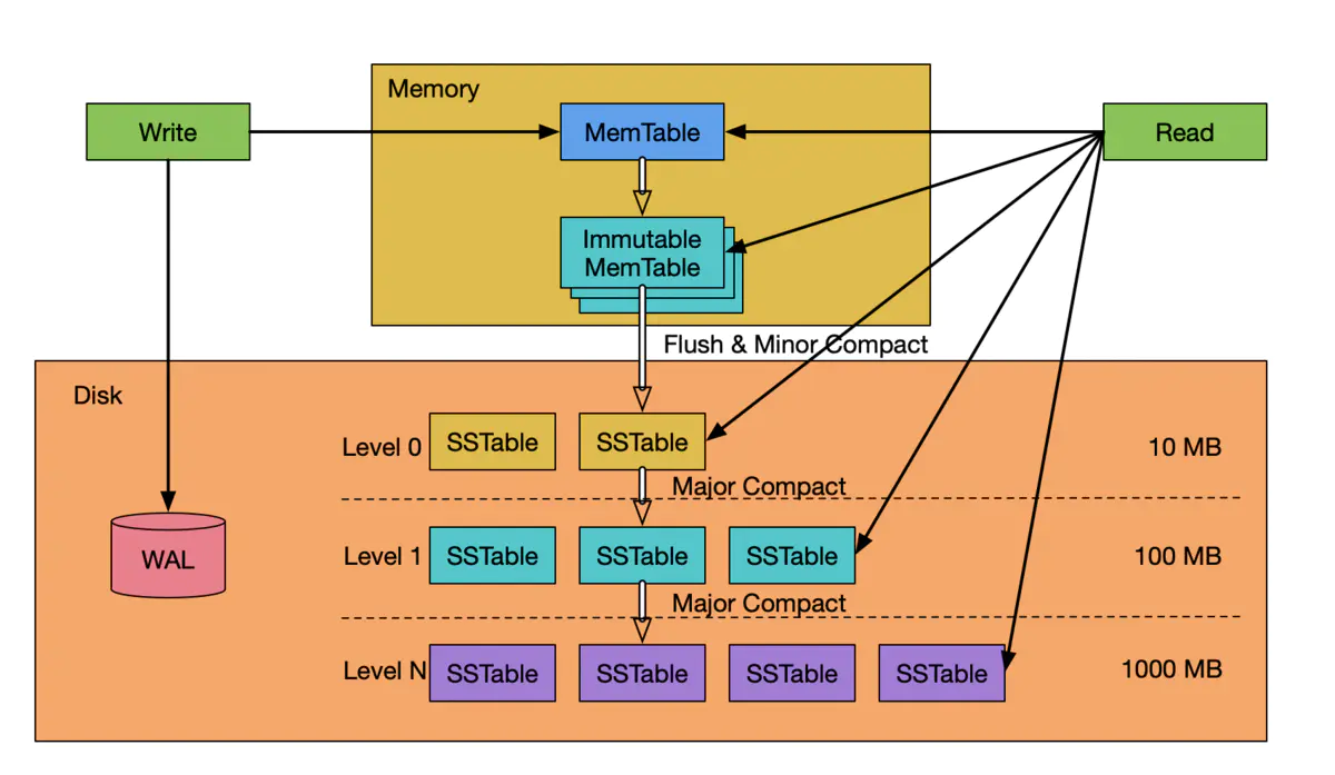
  The Log-Structured Merge-Tree was designed to solve the random write problem by converting all writes into fast, sequential I/O. The architecture is composed of several components:

  1. MemTable: A sorted, in-memory data structure (often a balanced binary tree or skip list). When a write request arrives, the data is written here first. Because this happens entirely in RAM, it's extremely fast.
  2. Write-Ahead Log (WAL): Simultaneously, the write is appended to a log file on disk. This is a sequential write and ensures durability. If the system crashes before the MemTable is saved, the WAL can be replayed to recover the data.
  3. SSTable (Sorted String Table): When the MemTable reaches a certain size threshold (e.g., 64MB), it is "frozen" (becomes an Immutable MemTable) and a new one is created for incoming writes. The full, immutable MemTable is then flushed to disk as a single, sorted, immutable file called an SSTable. This flush is a large, sequential write, which disks are highly optimized for.

  This entire process avoids random disk I/O for writes, making the LSM-Tree write path incredibly fast and capable of sustaining very high write throughput.

• Metaphor for a 5-Year-Old:
  An LSM-Tree write is like taking notes in a notebook.

  1. You write your newest notes on the current page (MemTable).
  2. Just in case you spill juice on your notebook, you have a separate piece of paper where you jot down everything you write as a backup (WAL).
  3. When the current page is full, you tear it out, label it "Page 1," and put it in a filing cabinet (SSTable). You then start writing on a fresh page. You never go back and erase things on the filed pages.

• Python Code Snippet:
  This code simulates a simple MemTable that flushes to a file when it gets full.

  import os
  import time
  
  class SimpleLSM:
      def __init__(self, data_dir="lsm_data", memtable_threshold=5):
          self.data_dir = data_dir
          self.memtable_threshold = memtable_threshold
          if not os.path.exists(self.data_dir):
              os.makedirs(self.data_dir)
          
          # In-memory component
          self.memtable = {}
          # On-disk WAL for durability (simplified)
          self.wal_file = open(os.path.join(self.data_dir, "wal.log"), "a")
  
      def set(self, key, value):
          print(f"Writing '{key}': '{value}'")
          # 1. Write to WAL first for durability
          self.wal_file.write(f"{key},{value}\n")
          self.wal_file.flush()
  
          # 2. Write to in-memory MemTable
          self.memtable[key] = value
  
          # 3. Check if MemTable should be flushed
          if len(self.memtable) >= self.memtable_threshold:
              print("--- MemTable full, flushing to SSTable on disk... ---")
              self.flush()
  
      def flush(self):
          # In a real system, this becomes an immutable memtable
          # and a new one is created.
          
          # Sort keys to create a Sorted String Table
          sorted_keys = sorted(self.memtable.keys())
          
          # Create a new SSTable file
          sstable_name = f"sstable_{int(time.time())}.db"
          sstable_path = os.path.join(self.data_dir, sstable_name)
          
          with open(sstable_path, "w") as f:
              for key in sorted_keys:
                  f.write(f"{key},{self.memtable[key]}\n")
          
          print(f"--- Flush complete. Created {sstable_name} ---")
          
          # Clear the MemTable for new writes
          self.memtable.clear()
      
      def close(self):
          self.wal_file.close()
  
  if __name__ == "__main__":
      db = SimpleLSM()
      db.set("user:3", "Charlie")
      db.set("user:1", "Alice")
      db.set("user:5", "Eve")
      db.set("user:2", "Bob")
      db.set("user:4", "David") # This write will trigger a flush
      db.set("user:6", "Frank") # This goes into the new, empty memtable
      db.close()
  

3. The LSM-Tree Read Path: The Price of Fast Writes (Medium)

• Technical Explanation:
  Herein lies the fundamental trade-off. Because data for the same key can exist in multiple places (the current MemTable and several SSTables on disk), a read operation is more complex than in a B-Tree. To find the value for a key, the system must search in reverse chronological order:

  1. Check the MemTable first. If the key is found, return the value.
  2. If not in the MemTable, check the most recent SSTable on disk.
  3. Continue checking older SSTables one by one until the key is found.
  4. If a key is not found after checking all SSTables, it doesn't exist.

  This process could require many disk reads, a phenomenon known as read amplification. To mitigate this, LSM-Trees use two key optimizations:

  • Bloom Filters: A probabilistic data structure stored with each SSTable. Before reading an SSTable file, the system asks its Bloom filter: "Does this file possibly contain this key?" A Bloom filter can say "definitely no" with 100% certainty, allowing the system to skip reading that file entirely. It might say "possibly yes" with a small false-positive rate, but it never has false negatives. This avoids most of the unnecessary disk reads for non-existent keys.
  • Sparse Indexes: SSTables also contain an index of some of the keys and their offsets in the file. This allows the system to seek to the approximate location of a key within the file rather than scanning the whole thing.

• Metaphor for a 5-Year-Old:
  You're trying to find the last thing you wrote about "dogs" in your notebook collection.

  • The Problem: You have to look at today's page, then yesterday's filed page, then the one from the day before... It could take a while.
  • The Bloom Filter: For each filed page, you attached a magic sticker. You can ask the sticker, "Does this page mention 'dogs'?" The sticker can instantly tell you "Nope, definitely not!" so you can skip it. If it says "Maybe," you have to read the page to be sure.
  • The Sparse Index: On each page, you wrote down in the margin where every 10th line starts. So instead of reading from the top, you can quickly jump to the right area of the page.

• Python Code Snippet (Conceptual):
  This conceptual function shows the logic of a read operation.

  # PSEUDOCODE for a read operation
  def get(key):
      # 1. Check the fast, in-memory MemTable first
      if key in memtable:
          return memtable[key]
  
      # 2. Check SSTables on disk, from newest to oldest
      for sstable in reversed(list_of_sstables):
          
          # Optimization 1: Check the Bloom Filter
          if key not in sstable.bloom_filter:
              # Key is definitely not in this file, skip it.
              continue 
          
          # Optimization 2: Use the sparse index to find the right block
          block_offset = sstable.sparse_index.find_offset(key)
          
          # Read the relevant block from disk
          data_block = read_disk_block(sstable.file, block_offset)
  
          # Scan the small block for the key
          value = data_block.find(key)
          if value is not None:
              # Found the most recent version of the key.
              return value
              
      # If we've searched everywhere and not found it
      return None
  

4. Compaction: Taming the Chaos (Hard)

• Technical Explanation:
  If SSTables were allowed to accumulate forever, read performance would degrade linearly. Compaction is the crucial background process that merges SSTables to control the read penalty. It reads several SSTables, merges their key-value pairs, discards overwritten or deleted values (tombstones), and writes the result into one or more new SSTables. This keeps the number of files to check during a read manageable.

  There are two primary compaction strategies:

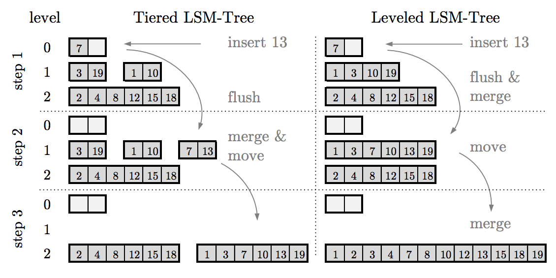
  • Size-Tiered Compaction (STCS): Merges several SSTables of a similar size into a new, larger SSTable in the next "tier". This is very efficient for the write path (low write amplification), but can lead to high space usage (space amplification) as multiple copies of a key may exist across different tiers for a while. Cassandra uses this strategy.
  • Leveled Compaction (LCS): Organizes SSTables into distinct levels (L0, L1, L2...). Level 0 can have multiple, overlapping files, but L1 and beyond each contain a single, large, sorted run of data. Compaction merges files from Level N with the overlapping keys in Level N+1. This results in lower read amplification and better space usage, but at the cost of higher write amplification, as data gets rewritten as it moves down the levels. RocksDB and LevelDB use this strategy.

• Metaphor for a 5-Year-Old:
  Compaction is like tidying up your collection of filed notebook pages.
  • Size-Tiered: You wait until you have five 1-page notes, then you merge them into a single 5-page document. Then you wait until you have five 5-page documents and merge them into a 25-page chapter.
  • Leveled: You have a strict system of folders. Your "Inbox" (L0) has a few pages. Once it has 5 pages, you merge them into your "Drafts" folder (L1). When the "Drafts" folder gets too big, you merge it into the "Final" folder (L2). This is more work, but it keeps everything very organized.

5. Amplification Factors: Quantifying the Trade-Offs (Harder)

• Technical Explanation:
  In system design interviews, you must be able to quantify the trade-offs of your architectural choices. For storage engines, we use three "amplification" metrics:

  1. Write Amplification: The ratio of bytes physically written to disk versus bytes written by the application. In an LSM-tree, this is primarily driven by compaction. If you write 1MB of data, but compaction rewrites it 10 times as it moves through the levels, the write amplification is 10x. This impacts disk throughput and the lifespan of SSDs. Leveled compaction generally has higher write amplification than tiered.
  2. Read Amplification: The number of disk I/O operations required to satisfy one read query. In an LSM-tree, this is the number of SSTables that must be checked to find a key. A worst-case read might check the MemTable and one SSTable at every level. Leveled compaction has lower read amplification because keys don't overlap within a level (except L0).
  3. Space Amplification: The ratio of disk space used versus the logical size of the data. This is caused by stale data (old versions of keys, deleted keys marked with tombstones) that hasn't been garbage collected by compaction yet. Tiered compaction generally has higher space amplification.

  The core trade-off is clear: LSM-Trees optimize for writes by accepting higher read and write amplification.

• Metaphor for a 5-Year-Old:
  Let's go back to our notebook analogy.
  • Write Amplification: You write one new sentence ("The dog is cute."). But to keep your notes organized, you have to re-copy the entire page with that new sentence added. You wrote one sentence, but physically copied 50. That's high write amplification.
  • Read Amplification: To find out what you wrote about the dog, you have to look at 3 different pages before you find the latest note. Your read amplification is 3.
  • Space Amplification: You have 10 pages of final notes, but you also have 20 pages of old drafts with crossed-out sentences that you haven't thrown away yet. The total space used is 30 pages. Your space amplification is 3x.

Conclusion

Today we've pulled back the curtain on the storage engine that makes many modern, large-scale data systems possible. You learned that the fundamental design of a data structure is a series of trade-offs, optimized for a specific access pattern.

Key Takeaways:

• LSM-Trees optimize for high write throughput by converting slow random disk writes into fast sequential writes using a MemTable and immutable SSTables.
• This optimization comes at a cost: a more complex read path that must check multiple files, leading to read amplification.
• Compaction is the essential background process that merges SSTables to manage read performance and reclaim disk space, but it introduces write amplification.
• Compaction strategies like Size-Tiered and Leveled offer different trade-offs between write, read, and space amplification, making them suitable for different workloads.
• Choosing between a B-Tree and an LSM-Tree is a critical system design decision based on whether the workload is read-heavy (favor B-Tree) or write-heavy (favor LSM-Tree).

Next Lesson Preview

We've seen how LSM-trees organize data for fast writes (OLTP-style). But what if your primary goal is fast analytical reads (OLAP-style), like calculating the average sales across millions of records? For that, a different storage layout is needed. In our next lesson, we will explore this by covering the learning outcome: Explain the benefits of columnar storage formats (e.g., Parquet) for analytical queries.