DP Complexity Analysis

1. A General Framework for DP Complexity Analysis

When analyzing a dynamic programming algorithm, the time complexity can almost always be determined by a simple formula.

As the resource states, the formula is:

Time Complexity = (Total number of unique subproblems) × (Time spent per subproblem)

Let's break this down:

• Number of Subproblems: This corresponds to the number of unique states your DP solution needs to solve. In a memoized solution, it's the number of distinct recursive calls you make (after pruning). In a tabulated solution, it's the number of entries in your DP table.
• Time per Subproblem: This is the work done within a single subproblem, assuming the solutions to any smaller subproblems it depends on are already known (either from the cache or the table). This usually involves looking up values and performing simple arithmetic or comparisons, which is often a constant time, $O(1)$, operation.

Space complexity is typically determined by two factors:

1. The storage needed for the DP table or memoization cache.
2. The maximum depth of the recursion stack (for memoized, top-down solutions).

Let's apply this framework to the examples we've seen.

2. Case Study: Fibonacci Sequence (1D DP)

The Fibonacci problem is a perfect starting point to see the dramatic impact of DP on complexity.

Brute-Force Recursion

First, consider the naive recursive solution without DP.

• Number of Subproblems: The recursion tree has a depth of $n$, and it branches twice at almost every node. This leads to an exponential number of nodes (subproblems), which is roughly $O(2^n)$.
• Time per Subproblem: The work inside the function is just an addition, which is $O(1)$.
• Time Complexity: $O(2^n)\times O(1)=O(2^n)$. This is extremely inefficient.
• Space Complexity: $O(n)$, determined by the maximum depth of the recursion call stack.

DP with Memoization (Top-Down)

Now, let's see what happens when we add a memoization cache.

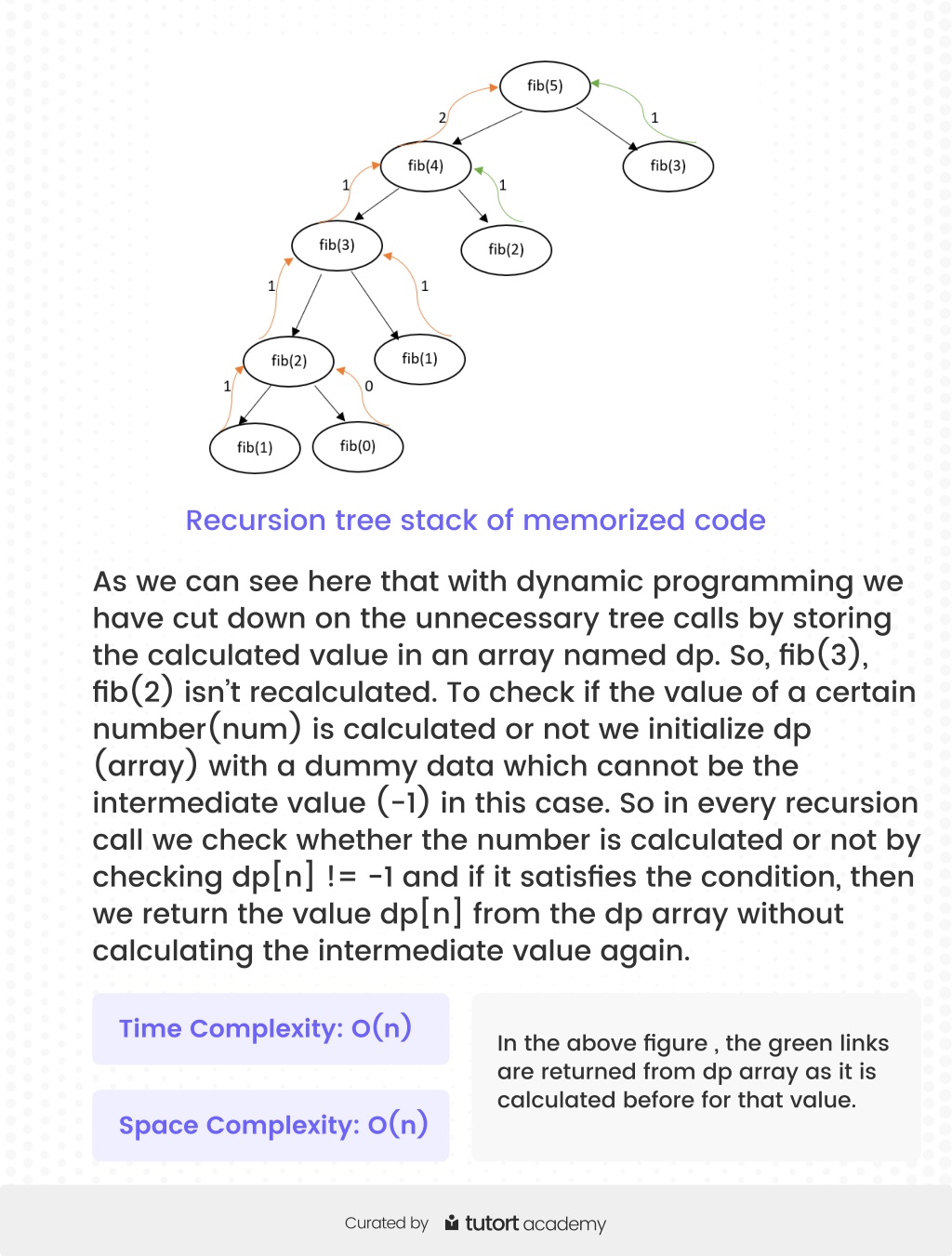
• Number of Subproblems: We only compute the value for each number from 0 to n once. So, there are n+1 unique subproblems. The number of subproblems is $O(n)$.
• Time per Subproblem: The work is still a simple addition, $O(1)$.
• Time Complexity: $O(n)\times O(1)=O(n)$. A massive improvement!
• Space Complexity: $O(n)$ for the memoization cache, plus $O(n)$ for the recursion stack depth. The total space is $O(n)$.

DP with Tabulation (Bottom-Up)

The analysis for the tabulated version is very similar.

• Number of Subproblems: We create a table of size n+1, so there are $O(n)$ subproblems (table entries) to fill.
• Time per Subproblem: Each entry is calculated with one addition, so the work is $O(1)$.
• Time Complexity: $O(n)\times O(1)=O(n)$.
• Space Complexity: $O(n)$ for the DP table. (Note: no recursion stack space is needed).

Finally, as we saw in the last lesson, the space for Fibonacci can be optimized to $O(1)$ by only keeping track of the last two values, while the time remains $O(n)$.

3. Case Study: 0/1 Knapsack Problem (2D DP)

Let's apply our framework to a 2D problem. In the 0/1 Knapsack problem, the state of a subproblem is defined by two parameters:

1. The number of items we are allowed to consider (let's say i, from 1 to N).
2. The remaining capacity of the knapsack (let's say w, from 1 to W).

Our DP state is dp[i][w].

Let's analyze it formally:

• Number of Subproblems: The DP table has N+1 rows (for items) and W+1 columns (for capacity). The total number of states or subproblems is $O(N\times W)$.
• Time per Subproblem: To compute dp[i][w], we perform a comparison and possibly an addition by looking up values in the previous row (dp[i-1][...]). This is an $O(1)$ operation.
• Time Complexity: $O(N\times W)\times O(1)=O(N\times W)$.
• Space Complexity: $O(N\times W)$ to store the entire DP table.

This analysis holds for both the tabulated and memoized versions. Remember from our last lesson that the space can be optimized to $O(W)$ by realizing we only need the previous row's data. However, the time complexity remains $O(N\times W)$ because we still have to solve all $N\times W$ subproblems.

An Important Note on Pseudo-Polynomial Time:
The complexity O(N * W) is called pseudo-polynomial time. It's polynomial in the value of the input W, but exponential in the size of the input W (which is log(W) bits). If W is extremely large, this algorithm can become slow. This is an advanced distinction but is fundamental to computational complexity theory and important from an architectural perspective.

4. Recognizing the Pattern

Let's look at one more example to solidify the pattern. For the Coin Change problem, where you need to find the minimum number of coins to make a certain amount given a set of k coin denominations:

• State: The subproblem is dp[a], the minimum coins for amount a. The states range from 1 to amount.
• Number of Subproblems: amount, so $O(\text{amount})$.
• Time per Subproblem: To compute dp[a], you might iterate through all k coins to see which one gives the best result. So the work per subproblem is $O(k)$.
• Time Complexity: $O(\text{amount}\times k)$.
• Space Complexity: $O(\text{amount})$ for the DP table.

You can see the framework holds consistently: identify the number of states and the work done per state.

Conclusion

Today you learned a formal method for analyzing the performance of your dynamic programming solutions. This moves you beyond just "making it work" and towards understanding the deep implications of your algorithmic choices.

Key Takeaways:

• The Golden Formula: Time Complexity in DP is typically (Number of Subproblems) × (Work per Subproblem).
• Subproblems are States: The number of subproblems is the number of entries in your DP table or unique calls in your memoized recursion.
• DP Reduces Complexity: DP transforms exponential-time brute-force solutions (like $O(2^n)$) into much more efficient polynomial-time solutions (like $O(n)$ or $O(n^2)$) by eliminating the redundant computation of overlapping subproblems.
• Space-Time Trade-offs: The default space complexity is usually proportional to the number of subproblems. However, as we've seen with Knapsack, you can often optimize space at the cost of implementation complexity, a classic architectural trade-off.

Preview of the Next Lesson:

Now that you can implement DP solutions with memoization and tabulation and analyze their complexity, it's time to put it all together. In our next lesson, we will do a deep dive into solving the 0/1 Knapsack problem from start to finish. We will apply the techniques from this module to a classic problem that is a cornerstone of many optimization challenges in software engineering.