Tabulation for Dynamic Programming

1. Tabulation vs. Memoization: Building from the Ground Up

In the previous lesson, we thought about solving problems by starting at the top (the main problem) and breaking it down recursively. Tabulation flips this idea on its head.

Tabulation is a bottom-up strategy. Instead of starting with the big problem, you start with the smallest, simplest subproblems (the base cases). You solve them first and store their results in a table (often an array or a 2D matrix). Then, you iteratively use these results to solve slightly larger subproblems, gradually building your way up until you arrive at the solution to the original problem.

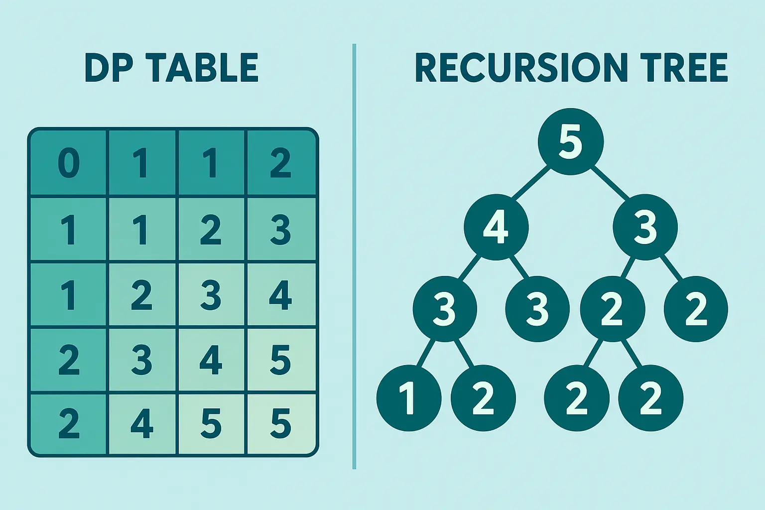
To solidify the distinction, let's look at a clear comparison.

As the resource highlights, the key difference is iteration vs. recursion. Tabulation replaces recursive calls with loops, which can lead to better performance in some programming languages due to the lack of function call overhead.

2. Implementing Tabulation: The Fibonacci Example

Let's revisit the Fibonacci sequence, which we solved with memoization last time. This will allow for a direct comparison of the two implementation styles.

The recurrence relation remains the same: $F(n)=F(n-1)+F(n-2)$.

To solve this with tabulation, we will:

1. Create a table (an array) of size n+1 to store the Fibonacci numbers.
2. Initialize the base cases: table[0] = 0 and table[1] = 1.
3. Iterate from i = 2 up to n, filling each entry table[i] by using the previously computed values: table[i] = table[i-1] + table[i-2].
4. The final answer is the value at table[n].

This process builds the sequence from the bottom (F(0), F(1)) all the way to the top (F(n)).

As the video explains, the complexity is:

• Time Complexity: $O(n)$. We iterate through the loop n-1 times, with each step being a constant time operation.
• Space Complexity: $O(n)$. We use an array of size n+1 to store our results.

This is the same complexity as the memoized solution, but we have achieved it iteratively.

3. A General Framework for Iterative DP

The Fibonacci example is straightforward. For more complex problems, like the 0/1 Knapsack or Longest Common Subsequence, having a systematic process is essential.

To summarize the key steps from the resource for creating a tabulation-based solution:

1. Initialize the Memoization Table: Create a data structure (e.g., a 1D or 2D array) to hold the solutions to all subproblems. Fill in the values for your base cases.
2. Iterate and Fill the Table: Design loops that iterate through the subproblems in an order that respects their dependencies. That is, when you compute the solution for a subproblem, the solutions for all the smaller subproblems it depends on must have already been computed. Inside the loops, apply your recurrence relation to calculate and store the result for each subproblem.
3. Return the Final Solution: The solution to the original problem will be one of the entries in your table (usually the last one).

4. Applying Tabulation to the 0/1 Knapsack Problem

Let's apply this framework to a more complex problem: the 0/1 Knapsack problem. As a reminder, you have a set of items, each with a weight and a value, and a knapsack with a maximum capacity. You want to choose items to maximize total value without exceeding the capacity.

The subproblem is defined by two parameters: the number of items considered and the current capacity.

• dp[i][w]: The maximum value achievable using a subset of the first i items with a knapsack capacity of w.

The recurrence relation is:

Let's build the iterative solution:

1. Initialize Table: Create a 2D table dp of size (num_items + 1) x (capacity + 1). The base cases are when i=0 (no items) or w=0 (no capacity), for which the value is 0. So, we can initialize the whole table to 0.

2. Iterate and Fill: The recurrence dp[i][w] depends on values from the previous row (i-1). This tells us our outer loop must be over the items (i), and the inner loop can be over the capacity (w).

   // dp table is initialized with zeros
   for i from 1 to num_items:
       for w from 1 to capacity:
           // Case 1: The current item is too heavy
           if weight[i-1] > w:
               dp[i][w] = dp[i-1][w]
           // Case 2: Decide whether to include the current item
           else:
               value_without_item_i = dp[i-1][w]
               value_with_item_i = value[i-1] + dp[i-1][w - weight[i-1]]
               dp[i][w] = max(value_without_item_i, value_with_item_i)
   

   (Note: we use weight[i-1] and value[i-1] because item i is at index i-1 in a 0-indexed array).

3. Return Result: The final answer is dp[num_items][capacity].

The time complexity is determined by the nested loops, which is $O(\text{num\_items}\times \text{capacity})$. The space complexity is for the table, which is also $O(\text{num\_items}\times \text{capacity})$.

5. A Critical Pitfall: Iteration Order and Space Optimization

The flexibility in loop order changes dramatically when we try to optimize space. For the knapsack problem, notice that to compute row i, we only ever need values from row i-1. We don't need rows i-2, i-3, etc. This suggests we can reduce our space complexity from $O(n\times C)$ to just $O(C)$ by using only two rows, or even just one!

However, if we use a single 1D array dp[w], the iteration order becomes paramount. This is a subtle but critical detail that separates a correct implementation from a buggy one.

As the resource explains, when using a 1D array dp[w], if you iterate the w loop from low to high, you end up using the same item multiple times within the same outer i loop. For example, when calculating dp[10] you might use dp[5], which was just updated using item i. This effectively solves the Unbounded Knapsack problem (where you have infinite copies of each item), not the 0/1 Knapsack problem.

By iterating the w loop backwards, from capacity down to weight[i], you ensure that when you calculate dp[w], the values like dp[w - weight[i]] are still from the previous i iteration (row i-1), thus correctly simulating the 2D table logic.

Conclusion

You have now learned the tabulation method, a powerful iterative approach to dynamic programming. You can see how it contrasts with the recursive memoization technique and where its strengths lie.

Key Takeaways:

• Tabulation is a bottom-up, iterative DP approach that builds solutions from base cases upwards.
• It avoids recursion, eliminating function call overhead and the risk of stack overflow, which can be an advantage for problems with very deep state dependencies.
• The implementation requires creating a DP table and filling it in an order that respects subproblem dependencies.
• When optimizing for space (e.g., reducing a 2D table to 1D), the iteration order can become critical to the correctness of the algorithm.

You now have both major DP implementation patterns in your arsenal. The choice between them is often a matter of context and preference, but knowing both allows you to select the most appropriate tool for the job.

Preview of the Next Lesson:

In the next lesson, we will formalize the process of analyzing the time and space complexity of a given DP solution. We'll also delve deeper into space optimization techniques, building on the concepts we touched upon today.