Crossing Symmetry and the Conformal Bootstrap

Hello! Welcome back to our exploration of Conformal Field Theory.

In our last lesson, we established a powerful tool: the decomposition of any four-point function into a sum over conformal blocks. This conformal partial wave expansion,

⟨ ϕ (x_{1}) ϕ (x_{2}) ϕ (x_{3}) ϕ (x_{4})⟩ = \frac{1}{∣ x _{12} ∣ ^{2 Δ_{ϕ}} ∣ x _{34} ∣ ^{2 Δ_{ϕ}}} O \sum C_{ϕϕ O}^{2} G_{Δ, ℓ} (u, v)

separated the theory-specific CFT data (the spectrum of primary operators ${Δ, ℓ}$ and their OPE coefficients $C_{ij k}$ ) from the universal kinematics encapsulated by the conformal blocks $G_{Δ, ℓ} (u, v)$ .

Today, we will address the central question: how do we constrain this unknown CFT data? The answer lies in a fundamental consistency condition that the Operator Product Expansion must satisfy: associativity. This single principle will lead us to the celebrated conformal bootstrap equations, a set of non-perturbative constraints that form the bedrock of the modern study of CFT.

OPE Associativity and Crossing Symmetry

The OPE allows us to compute a correlation function by repeatedly "fusing" operators. For a four-point function, there isn't a unique way to do this. We could fuse operators $(1, 2)$ and $(3, 4)$ , or we could fuse $(1, 4)$ and $(2, 3)$ , among other possibilities. The physical result—the value of the correlation function—must be independent of the order of fusion we choose. This is the essence of OPE associativity.

Equating the results from different fusion channels is known as imposing crossing symmetry.

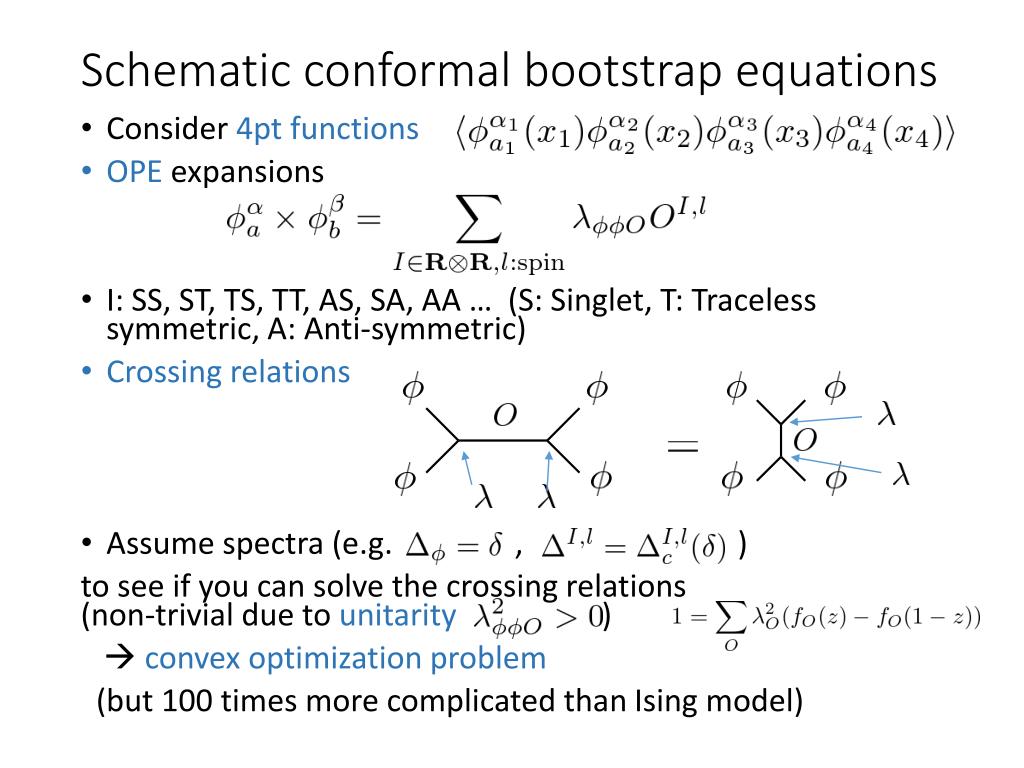
Schematic Conformal Bootstrap Equations — This diagram illustrates the core idea. The four-point function can be expanded by fusing operators in the s-channel (left) or the t-channel (right). Equating these two different expansions, which must be equal, leads to the bootstrap consistency condition, or crossing equation. The positivity of the OPE coefficients squared ($\lambda^2 > 0$) from unitarity is a crucial ingredient.

Let's formalize this. The expansion we derived in the last lesson corresponds to the s-channel, where we fuse $ϕ (x_{1}) ϕ (x_{2})$ and $ϕ (x_{3}) ϕ (x_{4})$ . Now, let's consider the t-channel, where we fuse $ϕ (x_{1}) ϕ (x_{4})$ and $ϕ (x_{2}) ϕ (x_{3})$ . This is equivalent to applying the s-channel expansion to the correlation function $⟨ ϕ (x_{1}) ϕ (x_{4}) ϕ (x_{2}) ϕ (x_{3})⟩$ . Since the operators are identical, this is just a permutation of the original correlator and must have the same value.

TASI Lectures on the Conformal Bootstrap

The following text from David Simmons-Duffin's TASI lectures articulates precisely how OPE associativity leads to the crossing symmetry equation for the four-point function.

Please read Section 10.1, "OPE Associativity and Crossing Symmetry" (pages 49-51). Focus on the core argument: the same correlation function can be computed in different ways by applying the OPE in different orders. The requirement that these computations agree yields the crossing symmetry equation. The diagram in equation (182) is the key takeaway.

As the reading explains, a CFT is fully specified by its data: the dimensions $Δ_{i}$ , spins $ℓ_{i}$ , and OPE coefficients $f_{ij k}$ (equivalent to our $C_{ij k}$ ). The requirement that the OPE is associative—that is, applying it in any order gives the same result—translates into a set of powerful constraints on this data, known as the crossing equations.

The Conformal Bootstrap Equation

Let's write down the crossing equation for a four-point function of identical real scalar primaries $ϕ$ with dimension $Δ_{ϕ}$ .

The s-channel expansion ( $12 \to 34$ ) is:

g (u, v) = O \sum (C_{ϕϕ O})^{2} G_{Δ, ℓ} (u, v)

where $g (u, v)$ is the four-point function stripped of its overall kinematic factor.

Now, consider the permutation $x_{1} \leftrightarrow x_{3}$ . The correlation function must be invariant. However, this permutation swaps the conformal cross-ratios: $u \leftrightarrow v$ . So, applying the same expansion logic after swapping $x_{1}$ and $x_{3}$ gives the t-channel expansion ( $32 \to 14$ ). Equating the two requires that the function $g (u, v)$ satisfies:

g (u, v) = (\frac{u}{v})^{Δ_{ϕ}} g (v, u)

Substituting the conformal block expansion into both sides gives the master equation:

O \sum (C_{ϕϕ O})^{2} G_{Δ, ℓ} (u, v) = (\frac{u}{v})^{Δ_{ϕ}} O \sum (C_{ϕϕ O})^{2} G_{Δ, ℓ} (v, u)

This can be rearranged into a more practical form. Let's define $p_{Δ, ℓ} = (C_{ϕϕ O})^{2}$ and move everything to one side:

Δ, ℓ \sum p_{Δ, ℓ} (v^{Δ_{ϕ}} G_{Δ, ℓ} (u, v) - u^{Δ_{ϕ}} G_{Δ, ℓ} (v, u)) = 0

This is the conformal bootstrap equation.

Weizmann Lectures on the Numerical Conformal Bootstrap

The following text from the "Weizmann Lectures on the Numerical Conformal Bootstrap" provides a very clear and concise summary of all the ingredients that go into the bootstrap equation for identical scalars.

Please read the beginning of Section 4, "Conformal bootstrap basics," and Section 4.1, "Bootstrap algorithms" (pages 37-38). Pay close attention to the list of properties in Section 4 and equation (4.5), which is the bootstrap equation written in a form ready for analysis.

As summarized in the reading, solving a CFT is equivalent to finding a consistent set of CFT data that satisfies this equation. The key constraints are:

The Spectrum: The sum is over primary operators with specific dimensions $Δ$ and spins $ℓ$ . In the OPE of two identical scalars, only even spin operators can appear. The spectrum must include the identity operator ( $Δ = 0, ℓ = 0$ ) and, for a local theory, the stress-energy tensor ( $Δ = d, ℓ = 2$ ).
Unitarity: For a unitary theory, the dimensions $Δ$ must obey the unitarity bounds we discussed previously. Crucially, unitarity also implies that the OPE coefficients are real, meaning their squares, $p_{Δ, ℓ} = (C_{ϕϕ O})^{2}$ , must be non-negative real numbers: $p_{Δ, ℓ} \geq 0$ .

This positivity constraint is the linchpin of the modern bootstrap program.

The Bootstrap Philosophy: From Equations to Bounds

The bootstrap equation is a single functional equation for an infinite number of unknowns ( $Δ, ℓ, p_{Δ, ℓ}$ ). Trying to find an exact solution is generally intractable. The breakthrough of the modern bootstrap, initiated in 2008 by Rattazzi, Rychkov, Tonni, and Vichi, was to instead ask: what spectra are inconsistent with this equation?

Let's rewrite the equation as:

Δ, ℓ \sum p_{Δ, ℓ} F_{Δ, ℓ} = 0, with p_{Δ, ℓ} \geq 0

Here, each $F_{Δ, ℓ}$ is a vector in the infinite-dimensional space of functions of $u$ and $v$ , defined as $F_{Δ, ℓ} (u, v) = v^{Δ_{ϕ}} G_{Δ, ℓ} (u, v) - u^{Δ_{ϕ}} G_{Δ, ℓ} (v, u)$ . The identity operator contributes a specific vector $F_{0, 0}$ . The equation states that the vector $F_{0, 0}$ must be expressible as a negative linear combination of all other vectors $F_{Δ, ℓ}$ with positive coefficients:

F_{0, 0} = - O \neq = 1 \sum \frac{p _{O}}{p _{1}} F_{Δ, ℓ}

This has a beautiful geometric interpretation. It means that the vector for the identity operator, $F_{0, 0}$ , must lie within the convex cone spanned by the negatives of the vectors for all other operators in the spectrum.

If we can find a hyperplane (defined by a linear functional $α$ ) that separates $F_{0, 0}$ from all the $- F_{Δ, ℓ}$ vectors allowed by a hypothetical spectrum, then that spectrum is ruled out.

TASI Lectures on the Conformal Bootstrap

Let's return to the TASI lectures for a clear conceptual explanation of this geometric approach to deriving bounds.

Please read Section 10.4, "Bounds on CFT Data" (pages 54-55). Focus on the logic behind Algorithm 1. The key idea is to assume a spectrum, which defines a set of vectors \vec{F}_{\Delta,\ell}, and then search for a linear functional \alpha that proves this assumption leads to a contradiction.

This procedure allows us to chip away at the space of possible CFT data. For instance, we can ask: "Is it possible to have a CFT where the lowest-dimension scalar operator appearing in the $ϕ \times ϕ$ OPE has a dimension $Δ_{0} > 5$ ?". We would then test this hypothesis by seeing if we can find a separating functional $α$ . If we can, that region of "theory space" is disallowed. By systematically testing such hypotheses, we can carve out allowed regions for operator dimensions and OPE coefficients.

Test your understanding!

Suppose you are bootstrapping a 3D CFT containing a scalar operator $ϕ$ . You make a hypothesis about the spectrum of operators appearing in the $ϕ \times ϕ$ OPE. You then run a numerical algorithm that successfully finds a linear functional $α$ such that:

$α (F_{0, 0}) = 1$ (a normalization choice).
$α (F_{Δ, ℓ}) \geq 0$ for all operators ${Δ, ℓ}$ in your hypothetical spectrum.

What can you conclude about your hypothetical spectrum? Is it consistent or inconsistent with the principles of CFT? Why?

Show answer

The hypothetical spectrum is inconsistent.

Here's why: The bootstrap equation is $\sum p_{Δ, ℓ} F_{Δ, ℓ} = 0$ . If we apply the linear functional $α$ to this equation, we get:

α (\sum p_{Δ, ℓ} F_{Δ, ℓ}) = \sum p_{Δ, ℓ} α (F_{Δ, ℓ}) = 0

Let's break down the sum. The identity operator's contribution is $p_{0, 0} α (F_{0, 0})$ . We can normalize the operator $ϕ$ such that $p_{0, 0} = 1$ , and the functional is normalized such that $α (F_{0, 0}) = 1$ . So this term is 1.

For all other operators, we know from unitarity that $p_{Δ, ℓ} \geq 0$ , and the functional was constructed such that $α (F_{Δ, ℓ}) \geq 0$ . Therefore, the sum over all other operators is a sum of non-negative terms.

= 1 p_{0, 0} α (F_{0, 0}) + \geq 0 O \neq = 1 \sum p_{Δ, ℓ} α (F_{Δ, ℓ}) = 0

This leads to the statement $1 + (a non-negative number) = 0$ , which is a contradiction. Therefore, the initial assumption about the spectrum must be false.

Conclusion

Today we have assembled the crown jewel of conformal invariance: the bootstrap equation. This is not just another formula; it represents a profound statement about the internal consistency of any quantum field theory with conformal symmetry.

Key Takeaways:

The associativity of the Operator Product Expansion (OPE) implies crossing symmetry for correlation functions.
For a four-point function, crossing symmetry leads to the conformal bootstrap equation, a functional equation that constrains the allowed spectrum $(Δ, ℓ)$ and OPE coefficients $(C_{ij k})$ of the theory.
The equation takes the form $\sum p_{i} V_{i} = 0$ , where $p_{i} = C_{i}^{2} \geq 0$ due to unitarity.
The modern bootstrap philosophy is not to solve this equation directly, but to use it to find bounds on CFT data by systematically ruling out inconsistent spectra.

We have now laid the complete groundwork for understanding CFTs as abstract mathematical structures. In our next lesson, we will begin to bridge the gap to the physical world. We will see how scale invariance at a second-order phase transition in a statistical mechanics system (like a magnet at its Curie temperature) is often enhanced to full conformal symmetry, allowing us to describe these critical phenomena using a CFT. The abstract operator dimensions $Δ$ we have been constraining will be identified with concrete, measurable critical exponents.

Recommended resources

OPE Associativity and Crossing Symmetry

The Conformal Bootstrap Equation

The Bootstrap Philosophy: From Equations to Bounds

Conclusion