Hello! Last lesson, you calculated why active power at the PCS terminals can differ from active power at the point of interconnection (POI). This lesson asks a different question: before accounting for the path to the POI, can a PCS produce the requested combination of active and reactive power at all?
You will read a supplied P–Q capability diagram, test operating points against its boundary, and distinguish an ideal MVA circle from the more detailed envelope a PCS supplier may provide. This completes the electrical foundation needed for later lessons on BESS operating limits and PPC commands.
Read the axes before the boundary
A P–Q diagram places an operating point using active power and reactive power . In the diagram below, positive means discharging toward the grid, while negative means charging from the grid. Positive means injecting reactive power; negative means absorbing it. These are the diagram’s conventions—not assumptions to carry over to every vendor chart or POI meter.
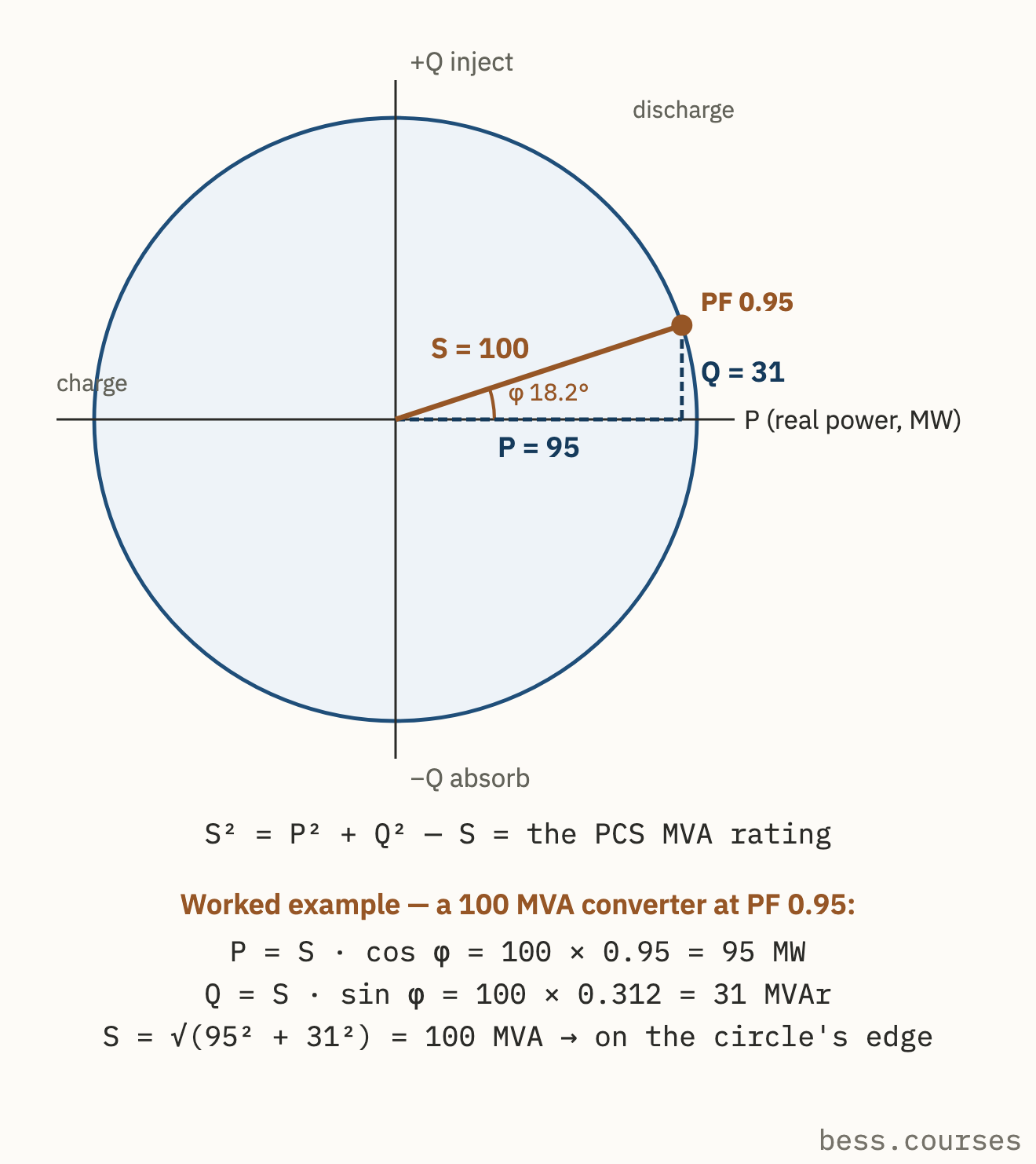
The shaded interior represents operating points permitted by this idealized apparent-power limit. The circle itself is the limit: a point on it uses the full stated MVA rating; a point outside it exceeds that rating. Its four regions also show something easy to miss in a charging discussion: charging does not determine the sign of reactive power. The PCS may, if its actual capability permits, inject or absorb reactive power while charging.
The marked point combines of discharge with roughly of reactive injection. It is not a request plus an independent allowance. Both components use the same apparent-power capacity.
Test a point against the MVA circle
For the circular diagram, the power triangle from the first lesson becomes a test for every proposed coordinate:
Here is in MW, in MVAr, and in MVA. With the diagram’s stated rating, the ideal-circle condition is
Because the signs disappear when squared, this particular circle is symmetric across both axes. That symmetry belongs to this diagram; it should not be presumed for every PCS.
Consider three proposed points under the diagram’s rated conditions:
| PCS request | Apparent power | Result against this circle |
|---|---|---|
| Inside | ||
| On the boundary | ||
| Outside |
The middle point is charging while absorbing reactive power. Its negative signs change the operating quadrant, but not the calculated MVA. The last point is infeasible under the stated limit even though each requested component, considered alone, is below .
You can also read the boundary as remaining headroom. At a specified active power, the largest reactive-power magnitude allowed by this ideal circle is
Thus, at either or , the circular limit leaves in either reactive direction. At , it leaves none. Conversely, if must be held, the largest active-power magnitude under this circle is . These are joint limits, not separate full-scale ratings.
The diagram’s power-factor point is consistent with the same test. At , , leaving
The figure rounds this to . A request for at power factor, however, would require . It would not fit this circle. “Rated MW” and “rated MVA” cannot be treated as interchangeable when reactive power is requested.
An actual capability envelope may be smaller
The circle answers one question: does the requested combination exceed the assumed apparent-power rating? A real PCS chart can impose additional boundaries. Available current depends on AC voltage; DC-side conditions, temperature, and equipment limits can also restrict sustained operation. Consequently, a point inside a nameplate MVA circle is not automatically inside the applicable supplier envelope.
Read the short explanation below with the ideal diagram in view. It distinguishes the simple circle from the conditional curves used for real equipment, and it distinguishes a PCS-terminal curve from a plant-level POI envelope.
What is the P-Q Capability Curve in BESS?
Read “What is the P-Q Capability Curve in BESS?” for its explanation of why the MVA circle is a starting point, not a complete operating guarantee.
Under “What it is, precisely,” read the first two paragraphs, beginning with the continuous MVA rating and ending with the discussion of curves at different AC voltages and temperatures. Then, in the same section, find the paragraph beginning “Three envelopes share the name.” Read from there through the POI distinction. Focus on which equipment, conditions, and measurement location each curve describes; you do not need the intervening product-specific numbers for this lesson.
A supplier chart may also put on the horizontal axis and on the vertical axis, or draw separate charging and discharging panels. Axis names, units, polarity notes, and reference location therefore come before any calculation. The following inverter presentation gives an example of those chart-reading details.
GE Energy Storage Inverter Capability Overview
Examine the “Capability Curve - Single Inverter” slide in the GE Energy Storage Inverter Capability Overview to see how a supplier presents charging and discharging limits under stated conditions.
Go to the slide labeled “Capability Curve - Single Inverter” and numbered 8. Start at its “Polarity convention” and condition notes; then inspect both plots, titled “Charging” and “Discharging,” through the voltage-trace labels beneath them. Notice that reactive power is labeled in kVar on the horizontal axis, active power in kW on the vertical axis, and the axes refer to the transformer secondary. Compare the different voltage traces without assuming that a point permitted on one trace is permitted on all of them.
This is why a feasibility statement should name its reference: feasible at which bus, at which voltage and temperature, under which available limits? A plotted boundary tells you what its stated conditions permit. It does not certify operation beyond those conditions.
Make a PPC-relevant feasibility decision
Suppose a PPC needs to assess a proposed PCS-terminal request. A reliable reading of the supplied diagram has four parts:
- Establish the coordinates. Identify the chart’s signs for charge, discharge, injection, and absorption, as well as the axis units. Convert units if necessary; do not compare kW directly with MW.
- Identify the applicable boundary. Select the curve for the stated operating conditions. If a detailed envelope is supplied, use its actual shape rather than replacing it with a nameplate circle.
- Locate the complete point. For a circle, calculate . For a noncircular supplied envelope, locate the intersection of the requested coordinates and check all nearby limits. Inside or on the stated boundary is permitted by that diagram; outside is not.
- State the conclusion at the diagram’s reference point. A feasible PCS-terminal request is not yet a proven feasible POI request. As the previous lesson showed for active power, intervening losses and loads matter. Reactive exchange through transformers and cables can matter too; translating the full envelope to the POI requires the project’s specified information.
That distinction prevents two opposite mistakes. The PPC must not request from the illustrated PCS merely because and . But it also should not reject a point on this ideal circle simply because charging has negative . The coordinates and the applicable boundary—not the sign of in isolation—settle the diagram-based question.
A final qualification is important: being inside a supplied steady-state P–Q envelope establishes feasibility only against the limits represented there. Battery availability or other current operating restrictions may narrow what the plant can deliver. The next module will examine those limits and which BESS systems have authority over them.
Key takeaways
A PCS operating point is a pair of active and reactive powers. On the supplied ideal circle, it is within the apparent-power limit when , using MW and MVAr. Increasing either power component uses capacity that could otherwise serve the other.
For a real feasibility decision, read the chart’s sign convention, units, reference bus, conditions, and actual boundary before testing the point. Keep a PCS-terminal conclusion separate from a POI capability claim. Next, you will build on this electrical picture by identifying the BESS components and controls that determine what the plant is currently allowed to do.