Modeling Triadic Emotional Influence in CLPMs

The Logic of Cross-Lagged Panel Models

At its core, a cross-lagged panel model (CLPM) is a type of structural equation model (SEM) designed to investigate reciprocal relationships between two or more variables measured at multiple time points. It simultaneously models two key processes:

1. Persistence (Autoregressive Effects): The tendency of a variable to be stable over time. This is captured by paths from a variable at one time point to the same variable at the next time point. For example, how predictive is the husband's jealousy at Time 1 of his jealousy at Time 2?
2. Influence (Cross-Lagged Effects): The hypothesized causal effect of one variable on another variable over time. This is the primary focus for causal inquiry. For example, what is the effect of the wife's guilt at Time 1 on the husband's jealousy at Time 2, holding the husband's prior jealousy constant?

This video provides an excellent high-level introduction to these core concepts.

To formalize this, we represent these relationships using a path diagram, a visual language for systems of linear equations. Your experience with DAGs in causal analysis will make this representation highly intuitive.

Visualizing the Model: The Bivariate Case

Let's start with the simplest case: modeling the dynamic interplay between the husband's jealousy (let's call it variable $y$) and the wife's guilt (variable $x$) across three time points, as collected by your ESM protocol.

The path diagram for this model would look like this:

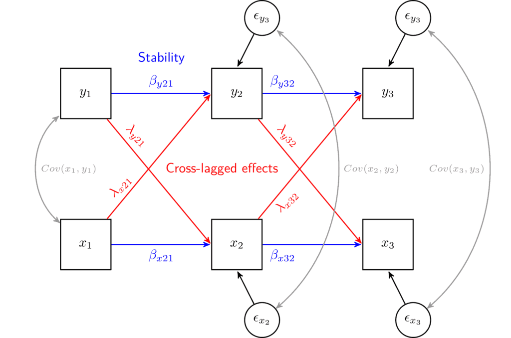
Let's decode this diagram:

• Variables: The squares represent the observed variables at each time point (e.g., $y_1$ is husband's jealousy at Time 1, $x_2$ is wife's guilt at Time 2).
• Stability Paths (Autoregressive): The blue arrows, like the one from $y_1$ to $y_2$ with coefficient ${\beta }_{y21}$, estimate the stability of husband's jealousy. A large, positive $\beta$ means jealousy is highly persistent.
• Influence Paths (Cross-Lagged): The red arrows, like the one from $x_1$ to $y_2$ with coefficient ${\lambda }_{x21}$, estimate the influence of the wife's guilt at Time 1 on the husband's jealousy at Time 2. This is the key parameter for your causal hypothesis.
• Contemporaneous Covariances: The curved grey arrows, like the one between $x_1$ and $y_1$, represent the correlation between the two variables at the initial time point. The similar curves between the error terms ($ϵ$) at later time points (e.g., between $y_2$ and $x_2$) account for any shared influences or covariation at that moment that isn't explained by the model's lagged predictors.

Specifying the Triadic CLPM

Your research involves a triad, so we must expand this model. Let's define our three core emotional variables:

• $H_t$: Husband's Jealousy at time $t$
• $W_t$: Wife's Guilt at time $t$
• $B_t$: Bull's Emotional Detachment at time $t$

To specify the triadic CLPM, we simply extend the logic from the bivariate case. For each step in time (e.g., from $t$ to $t+1$), our model will include:

• Three Autoregressive Paths: These capture the stability of each person's emotion.

  • $H_t\to H_{t+1}$
  • $W_t\to W_{t+1}$
  • $B_t\to B_{t+1}$

• Six Cross-Lagged Paths: These capture all possible directions of influence between the three participants.

  • $W_t\to H_{t+1}$ (Wife's guilt influencing Husband's jealousy)
  • $B_t\to H_{t+1}$ (Bull's detachment influencing Husband's jealousy)
  • $H_t\to W_{t+1}$ (Husband's jealousy influencing Wife's guilt)
  • $B_t\to W_{t+1}$ (Bull's detachment influencing Wife's guilt)
  • $H_t\to B_{t+1}$ (Husband's jealousy influencing Bull's detachment)
  • $W_t\to B_{t+1}$ (Wife's guilt influencing Bull's detachment)

• Three Contemporaneous Covariances: The error terms for $H_{t+1}$, $W_{t+1}$, and $B_{t+1}$ are allowed to covary. This is crucial because any shared event at time $t+1$ (e.g., a specific conversation) could simultaneously affect all three participants' emotions in ways not captured by the lagged effects.

The system of equations for predicting the emotions at time $t+1$ would be:

This complete specification captures the full, complex web of potential emotional influences within your triad over time. The following reading explains how such multivariate panel models are conceived within the SEM framework and how they can be extended.

A Critical Refinement: Isolating Within-Person Effects

Your goal is causal inference. You want to know if a change in one person's emotional state causes a subsequent change in another's. A standard CLPM, as specified above, has a significant vulnerability: it conflates within-person change with stable between-person differences.

For example, a positive cross-lagged path from wife's guilt to husband's jealousy could mean two very different things:

1. Within-person process (causal): When this specific wife feels more guilty than she usually does, her husband becomes more jealous than he usually does at the next time point.
2. Between-person correlation (spurious): Couples where the wife is, on average, a more guilt-prone person also tend to be couples where the husband is, on average, a more jealousy-prone person.

The standard CLPM cannot distinguish between these two interpretations. To isolate the true within-person causal process, we must explicitly model the stable, between-person differences. This is achieved by specifying a Random Intercept Cross-Lagged Panel Model (RI-CLPM).

The RI-CLPM adds a latent random intercept for each person's emotional variable. This intercept represents that person's stable, trait-like mean level of that emotion over the course of the study. By including these intercepts, the cross-lagged paths are estimated based on the deviations from each person's own average. This effectively "person-mean centers" the data, allowing the cross-lagged coefficients to be interpreted as true within-person effects.

The following video masterfully explains this problem and presents the RI-CLPM solution.

For your triadic study, specifying an RI-CLPM means you would add three latent random intercepts: one for Husband's Jealousy, one for Wife's Guilt, and one for Bull's Detachment. These intercepts would be allowed to correlate, capturing the stable, between-triad differences in the overall emotional climate. The cross-lagged paths would then give you a much cleaner estimate of the dynamic, within-triad causal influences.

Conclusion

In this lesson, we have moved from the abstract need to model longitudinal influence to the concrete specification of a triadic cross-lagged panel model. You now understand the components of this model and how to represent them visually and mathematically. Most importantly, you have learned the critical distinction between a standard CLPM and the more causally robust Random Intercept CLPM.

Key Takeaways:

• A CLPM decomposes longitudinal relationships into autoregressive paths (stability) and cross-lagged paths (influence).
• A triadic CLPM can be specified to model the full set of 3 stability paths and 6 reciprocal influence paths among the husband, wife, and bull.
• Path diagrams are the conventional language for specifying the system of equations that constitute the model.
• The Random Intercept CLPM (RI-CLPM) is the modern standard for causal inference with panel data, as it separates stable between-person differences from the dynamic within-person processes you aim to study.

You have now specified the theoretical structure of your primary analytical tool. In our next lesson, we will bring this model to life by discussing how to estimate and interpret the autoregressive and cross-lagged path coefficients from a fitted CLPM, allowing you to finally answer the directional questions about emotional influence in the triad.