Hello! Welcome to our next lesson on Spreadsheet Essentials.
In our last session, we mastered how to merge cells to create clean, professional-looking titles and headings for our accounting reports. We learned that this is a key skill for improving the layout and readability of a spreadsheet.
Today, we're shifting our focus from the structure of the sheet to the data itself. A raw number like 50000 is ambiguous. Is it a quantity, or is it ₹50,000? Likewise, 0.08 is harder to read than 8%. Our goal for this lesson is to learn how to apply various number formatting tools, including currency, percentages, and dates, to make our financial data clear, professional, and instantly understandable. This is a fundamental skill that is frequently tested.
1. Why Number Formatting Matters in Accounting
Before we dive into the "how," let's quickly establish the "why." In accounting, precision and clarity are non-negotiable. Proper formatting ensures that anyone reading your spreadsheet—be it a manager, an auditor, or an exam evaluator—interprets the numbers exactly as intended.
Consider this raw data:
| Item | Value |
|---|---|
| Sales | 150000 |
| Tax | 0.05 |
| Date | 45383 |
Now, look at the same data with formatting applied:
| Item | Value |
|---|---|
| Sales | ₹ 1,50,000.00 |
| Tax | 5.00% |
| Date | 01-Apr-2024 |
The second table is immediately clearer and more professional. This transformation is what we'll learn to do today.
2. Finding Your Formatting Toolkit
The primary tools for number formatting are conveniently located on the Home tab of the Excel ribbon, within the Number group.
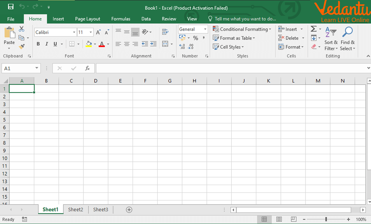
3. A Deep Dive into Formatting Options
While the ribbon buttons are great for quick changes, the Format Cells dialog box gives you complete control. You can access it by clicking the small arrow in the bottom-right corner of the Number group, or by right-clicking a cell and choosing "Format Cells...".
Let's explore the specific formats you need for your exam using the official NCERT textbook content.
[PDF] ACCOUNTANCY - Knowledge Gallery
This PDF from your core textbook provides a detailed, step-by-step guide to applying number formats. It explains how to use the Format Cells dialog box to apply Currency, Percentage, and other special formats.
Please read section 2.3 DATA FORMATTING and subsection 2.3.1 FORMATTING TOOLS. Focus specifically on the parts describing: Number formatting in general. The examples for applying Currency and Percentage formats (referencing Figures 2.52a through 2.52d). The brief description of how Dates are handled.
4. Applying Key Formats: A Step-by-Step Guide
Based on the textbook and common spreadsheet practice, let's consolidate the steps for the three most important formats for accounting.
A. Currency Format
This is used for all monetary values, like sales, expenses, and profits.
- Quick Method: Select the cells and click the Accounting Number Format button (often a '$' or '₹' symbol) in the Number group.
- Detailed Method (
Format Cellsbox):- Select the cell(s) you want to format.
- Right-click and choose Format Cells....
- Go to the Number tab and select the Currency or Accounting category. (For financial reports, Accounting is often preferred as it aligns currency symbols and decimal points neatly in a column).
- Choose the desired Symbol (e.g., ₹ for Indian Rupee).
- Set the number of Decimal places (typically 2 for financial values).
- Click OK.
B. Percentage Format
This is used for ratios, growth rates, and tax rates.
- Quick Method: Select the cells and click the Percent Style (%) button in the Number group.
- Important Note: Excel multiplies the cell value by 100 when you apply the percentage format. To display
25%, you must either enter the decimal0.25or type25%directly into the cell. If you type25and then apply the format, you will get2500%. - Detailed Method (
Format Cellsbox):- Select the cell(s).
- Open the Format Cells dialog box.
- Under the Number tab, choose the Percentage category.
- Specify the number of Decimal places you need.
- Click OK.
C. Date Format
This is crucial for recording transaction dates, report dates, and deadlines.
- How Excel Handles Dates: As you read, Excel is smart enough to recognize entries like
16/04/2024or16-Apr-2024as dates. Internally, it stores them as serial numbers, which allows you to perform calculations with them (e.g., finding the number of days between two dates). - Detailed Method (
Format Cellsbox):- Enter your date in a recognizable format.
- Select the cell(s).
- Open the Format Cells dialog box.
- Under the Number tab, choose the Date category.
- Select the desired format from the Type list (e.g.,
dd-mm-yyyy,dd-mmm-yy,mmmm d, yyyy). - Click OK.
For a quick look at how Excel can automatically generate dates using functions, this short video is helpful.
Computerized Accounting | SPREADSHEET | Class-12 | ISC | Section C | Accounts | Shubham Jagdish
While our main focus is formatting existing data, it's also useful to see how Excel can create dates with functions. This video from SHUBHAM JAGDISH briefly touches upon date and time functions.
Watch the segment from 00:49:09 to 00:50:21. The instructor explains functions like TODAY(), NOW(), and DATEVALUE(), which are related to working with dates in a spreadsheet.
Exam-Style Practice
Let's apply what you've learned.
Question: You are preparing a Sales Report in a spreadsheet with the following columns: Date, Product, Units Sold, Sale Price, Total Revenue, and GST Rate (as a decimal). Describe the specific number format you would apply to the Date, Sale Price, Total Revenue, and GST Rate columns to ensure the report is clear and professionally presented.
Model Answer:
- Date Column: I would apply a Date format, specifically
dd-mm-yyyy, to ensure all dates are displayed consistently and unambiguously. - Sale Price Column: I would apply the Accounting format, set the currency symbol to
₹, and use 2 decimal places. This is appropriate for monetary values. - Total Revenue Column: Similar to Sale Price, I would apply the Accounting format with the
₹symbol and 2 decimal places to clearly represent the total monetary value of the sales. - GST Rate Column: I would apply the Percentage format with 2 decimal places. This will convert decimal values (e.g., 0.18) into a more readable format (18.00%).
Conclusion
In this lesson, you've learned how to transform raw numbers into meaningful financial information using essential formatting tools. Mastering these techniques is not just about making your spreadsheet look good; it's a core competency for accurate and professional computerized accounting.
Key Takeaways:
- Number formatting is crucial for clarity and professionalism in accounting reports.
- The primary tools are in the Number group on the Home tab.
- The Format Cells dialog box provides advanced control over formats like Currency, Percentage, and Date.
- Choosing the right format (e.g., Currency/Accounting for money, Percentage for rates, Date for timelines) prevents misinterpretation of data.
In our next lesson, we will step back slightly to cover a very basic but critical concept: identifying the difference between the active cell and the active worksheet. Understanding this distinction is fundamental to navigating and manipulating data effectively in any spreadsheet application.