Understanding Modes of Convergence

Introduction

Welcome to your course on advanced statistics! Given your background in theoretical physics and mathematics, we will take a rigorous path through the material, focusing on the core concepts that underpin modern statistical theory. We'll begin our journey in this first module with the fundamental language of large-sample theory: the convergence of random variables.

This lesson introduces three key ways in which a sequence of random variables can converge: convergence in probability, almost sure convergence, and convergence in distribution. Understanding the precise meaning of each and the relationships between them is essential for making sense of the major results in statistics, such as the Law of Large Numbers and the Central Limit Theorem. These concepts provide the mathematical foundation for understanding why statistical methods work as we collect more data.

An Intuitive Overview

Before we dive into formal definitions, let's build some intuition. Many of the most important theorems in statistics describe the limiting behavior of sample statistics as the sample size grows. However, the term "converges" can mean different things in a probabilistic context.

To get a feel for these different flavors of convergence, please watch the first part of the following lecture from Harvard's Statistics 110 course. It introduces the Law of Large Numbers and the Central Limit Theorem, which are prime examples of where these different modes of convergence appear.

Lecture 29: Law of Large Numbers and Central Limit Theorem | Statistics 110

This video by Professor Joe Blitzstein provides an excellent intuitive introduction to the different ways a sample mean can converge to a true mean. Pay close attention to his distinction between the 'strong' and 'weak' laws, and how the Central Limit Theorem describes convergence in a different sense.

Please watch the video from the beginning until 21:57. Focus on how the lecturer informally describes: Strong Law of Large Numbers: Convergence 'with probability 1' (this is almost sure convergence). Weak Law of Large Numbers: The probability of being far from the mean goes to zero (this is convergence in probability). Central Limit Theorem: Convergence 'in distribution' to the normal distribution.

As you saw, these theorems make precise statements about the long-run behavior of the sample mean, but they rely on different notions of what "long-run behavior" means. Let's now formalize these ideas.

Formal Definitions of Convergence

We will now define the three main modes of convergence. For these concepts to be relevant, we consider a sequence of random variables $X_{1}, X_{2}, \dots$ and a limiting random variable $X$ , which are all defined on the same underlying probability space.

1. Convergence in Probability

This mode of convergence formalizes the idea that it becomes increasingly unlikely for $X_{n}$ to be far from $X$ as $n$ grows. This corresponds to the Weak Law of Large Numbers discussed in the video.

Definition: A sequence of random variables $X_{n}$ converges in probability to a random variable $X$ , written $X_{n} p X$ , if for every $ϵ > 0$ ,

n \to \infty lim P (∣ X_{n} - X ∣ \geq ϵ) = 0

Intuitively, this means that for a large enough $n$ , the probability of $X_{n}$ and $X$ differing by more than any small, fixed amount $ϵ$ becomes negligible. However, this does not rule out the possibility that for any given outcome $ω$ , the sequence of values $X_{n} (ω)$ might occasionally make large jumps away from $X (ω)$ .

2. Almost Sure Convergence

Almost sure convergence is a stronger condition. It requires that the sequence of outcomes $X_{n} (ω)$ converges to $X (ω)$ in the same way a sequence of real numbers does, for all outcomes $ω$ except for a set of "bad" outcomes that has probability zero. This corresponds to the Strong Law of Large Numbers.

Definition: A sequence of random variables $X_{n}$ converges almost surely (or with probability 1) to a random variable $X$ , written $X_{n} a . s . X$ , if

P ({ω : n \to \infty lim X_{n} (ω) = X (ω)}) = 1

The connection to your mathematical background in analysis is that almost sure convergence of random variables is the probabilistic analog of pointwise convergence of functions almost everywhere.

For a more detailed, formal construction of this definition, the following video may be of interest.

Master Program: Probability Theory - Lecture 4: Convergence of random variables

This lecture from IMPA provides a rigorous, step-by-step construction of the formal definition of almost sure convergence, translating the limit of a sequence of functions into a statement about probabilities of nested sets. This might appeal to your mathematical background.

Watch the segment from 00:05 to 12:19. The key idea is to see how the statement 'for all epsilon, there exists an N...' is translated into intersections and unions of events, which allows us to use the axioms of probability.

3. Convergence in Distribution

This is the weakest form of convergence. It states that the cumulative distribution function (CDF) of $X_{n}$ converges to the CDF of $X$ . It only concerns the "shape" of the distributions, not the random variables themselves. In fact, the variables $X_{n}$ and $X$ need not even be defined on the same probability space. This is the mode of convergence in the Central Limit Theorem.

Definition: A sequence of random variables $X_{n}$ with CDFs $F_{n}$ converges in distribution to a random variable $X$ with CDF $F$ , written $X_{n} d X$ , if

n \to \infty lim F_{n} (x) = F (x)

for every point $x$ at which $F$ is continuous.

The condition "at which $F$ is continuous" is a technical requirement to handle convergence to discrete random variables properly.

The Hierarchy of Convergence

These three modes of convergence are not independent; they are related in a clear hierarchy. To explore this, please read the following sections from the MIT OpenCourseWare notes.

Convergence of Random Variables - MIT OpenCourseWare

These notes formally define the three modes of convergence and then explicitly state and prove the relationships between them. This will solidify your understanding of how they differ in strength.

Please read the following parts of the document: Section 1.1 'Almost sure convergence' Section 1.2 'Convergence in distribution' Section 1.3 'Convergence in probability' Section 3 'THE HIERARCHY OF CONVERGENCE CONCEPTS' Focus on Theorem 5, which summarizes the implications, and the counterexamples in Sections 3.1 and 3.2 that show why the reverse implications do not hold.

The key takeaways from this reading are summarized by the following relationships:

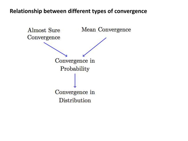
Relationship between Different Types of Convergence — A diagram illustrating the hierarchy of convergence modes. 'Mean Convergence' (or L_p convergence) is another mode that we will not focus on in this lesson, but as shown, it also implies convergence in probability.

In short:

(X_{n} a . s . X) ⟹ (X_{n} p X) ⟹ (X_{n} d X)

Let's break this down:

Almost Sure $⟹$ In Probability: If the sequence of values converges for almost every outcome, then the probability of a large deviation at a specific $n$ must necessarily go to zero. The reverse is not true. A classic counterexample involves a "sweeping" probability mass that ensures convergence in probability to zero, but since every point is "hit" infinitely often, the sequence does not converge almost surely.
In Probability $⟹$ In Distribution: If the probability mass of $X_{n}$ concentrates around $X$ , then their CDFs must also converge. The reverse is not true, unless the limit is a constant. For example, if you let $X$ be a standard normal random variable and set $X_{n} = - X$ for all $n$ , then $X_{n}$ has the same distribution as $X$ for all $n$ , so $X_{n} d X$ . However, $P (∣ X_{n} - X ∣ > ϵ) = P (∣ - 2 X ∣ > ϵ)$ , which is a fixed positive probability, not zero. So $X_{n}$ does not converge in probability to $X$ .

An Important Special Case:
As mentioned in the notes, convergence in distribution does imply convergence in probability if the limit is a constant, $c$ .

(X_{n} d c) ⟺ (X_{n} p c)

This is an extremely useful result that is frequently used in proofs.

A Practical Example

Let's solidify these ideas with an exercise. Consider a sequence of independent random variables $X_{n}$ defined on the interval $[0, 1]$ with a uniform probability measure, such that:

X_{n} = {10 with probability 1/ n with probability 1 - 1/ n

Does this sequence converge to 0? In which modes?

Click to see the analysis

Convergence in Probability:
For any $ϵ > 0$ (e.g., $ϵ = 0.5$ ), we check the definition:
$P (∣ X_{n} - 0∣ \geq ϵ) = P (X_{n} = 1) = \frac{1}{n}$
Since $lim_{n \to \infty} \frac{1}{n} = 0$ , we can conclude that $X_{n} p 0$ .
Almost Sure Convergence:
For almost sure convergence, we need the sequence of outcomes $X_{n} (ω)$ to converge to 0 for almost all $ω$ . This means that for any given $ω$ , $X_{n} (ω)$ should be 0 for all $n$ larger than some $N (ω)$ . In other words, the event ${X_{n} \neq = 0}$ should occur only a finite number of times.
We can check this using the Borel-Cantelli lemmas. The sum of the probabilities is:
$\sum_{n = 1}^{\infty} P (X_{n} \neq = 0) = \sum_{n = 1}^{\infty} \frac{1}{n} = \infty$
Since the $X_{n}$ are independent and the sum of probabilities diverges, the second Borel-Cantelli lemma states that $P (X_{n} \neq = 0 infinitely often) = 1$ .
This means that with probability 1, the sequence $X_{n} (ω)$ will contain an infinite number of 1s and thus does not converge to 0. Therefore, $X_{n}$ does not converge almost surely to 0.
Convergence in Distribution:
Since convergence in probability implies convergence in distribution, we know that $X_{n} d 0$ . We can also check this directly from the CDF. The CDF of $X_{n}$ is:
$F_{n} (x) = ⎩ ⎨ ⎧ 0 1 - 1/ n 1 if x < 0 if 0 \leq x < 1 if x \geq 1$
The CDF of the constant random variable $X = 0$ is $F (x) = 0$ for $x < 0$ and $F (x) = 1$ for $x \geq 0$ . As $n \to \infty$ , $F_{n} (x)$ converges to $F (x)$ at all points except the discontinuity at $x = 0$ . By definition, this means $X_{n} d 0$ .

Conclusion

In this lesson, we have defined and distinguished the three primary modes of stochastic convergence.

Key Takeaways:

Convergence in Distribution ( $X_{n} d X$ ): The CDF of $X_{n}$ approaches the CDF of $X$ . This is the weakest form of convergence.
Convergence in Probability ( $X_{n} p X$ ): The probability that $X_{n}$ is far from $X$ becomes vanishingly small.
Almost Sure Convergence ( $X_{n} a . s . X$ ): The sequence of random variables converges to $X$ for all outcomes except a set of probability zero. This is the strongest form.
The relationships form a strict hierarchy: Almost Sure $⟹$ In Probability $⟹$ In Distribution. The converses are not generally true, with the important exception that convergence in distribution to a constant is equivalent to convergence in probability to that constant.

These concepts form the essential grammar for the limit theorems we will explore next.

Preview of the Next Lesson:

In the next lesson, we will apply these concepts to one of the cornerstones of probability and statistics: the Law of Large Numbers. We will formally state and prove the Weak Law of Large Numbers (using convergence in probability) and discuss the Strong Law of Large Numbers (using almost sure convergence).

Recommended resources