Hello! Welcome to the first lesson in our new module, "Analyzing Algorithm Efficiency."
In the previous modules, you've built a solid foundation in programming, from the basics of Python to the principles of Object-Oriented Programming. You've learned how to write code that works and how to structure it well. Now, we're going to shift our focus from making it work to making it work well.
Your goal for this lesson is to explain why measuring algorithm efficiency is critical for large inputs. This is a cornerstone of computer science and a crucial skill for technical interviews. We won't be measuring anything just yet; first, we need to understand why it's so important to do so.
1. How Fast Is My Code? Why Not Just Use a Stopwatch?
Imagine you've written a program. A natural first question is, "How fast is it?" The most intuitive way to answer this might be to run the code and time it, like using a stopwatch.
However, this approach has some serious flaws. What if you run the program on a brand-new, powerful gaming computer versus a ten-year-old laptop? The results would be vastly different, but that's a reflection of the hardware, not the quality of your algorithm.
Let's start with a short article that clearly lists these problems.
The article 'Algorithm Complexity Analysis PART I - Big O' by João Godinho on DEV Community gives a concise breakdown of why simply timing your code isn't a reliable way to measure its efficiency.
Read the first two bulleted lists under the heading 'What does Asymptotic and Asymptotic Notation mean?'. Focus on the points that explain the problems with direct measurement and why we need a machine-independent way to evaluate algorithms.
The article highlights that results can vary between computers and even on the same computer depending on what else is running. To be effective problem-solvers, we need a consistent way to talk about an algorithm's performance, regardless of the machine it runs on.
The next video demonstrates this exact point.
Introduction to Big O Notation and Time Complexity (Data Structures & Algorithms #7)
In this clip from 'Introduction to Big O Notation' by CS Dojo, the instructor runs the same code on two different computers to show how timing can be misleading.
Watch from 11:23 to 12:29. Notice how the execution times differ between the two machines. The key takeaway is that even though one computer is faster, the growth in time as the input gets bigger follows a similar pattern on both. This is the pattern we want to analyze.
This leads us to a crucial conclusion: we're not interested in the exact number of seconds an algorithm takes. We're interested in how its runtime changes as the size of the input grows.
2. The Importance of Scale: From 10 to 10 Million
The difference between a good algorithm and a bad one is barely noticeable for small inputs. If you're sorting a list of 10 numbers, almost any method will feel instantaneous. But what if you need to sort a list with 10 million numbers? This is where efficiency becomes critical.
In today's world, we deal with enormous datasets. Think about Google searching trillions of web pages, or scientists analyzing the human genome, which contains billions of data points. A small inefficiency in an algorithm can be the difference between getting an answer in a second and waiting for a year.
Let's watch a segment from an MIT lecture that puts this into perspective.
10. Understanding Program Efficiency, Part 1
Professor John Guttag from MIT OpenCourseWare explains why efficiency matters more than ever, even with today's incredibly fast computers.
Watch the segment from 05:07 to 06:51. Pay attention to the examples of Google search and genomics data. These illustrate how the size of problems we want to solve is growing so rapidly that we can't just rely on faster hardware.
As the video explains, the datasets are growing so fast that even with faster computers, we need efficient algorithms.
The graph below provides a powerful visual for this concept. It shows how the number of operations (which relates to time) for different types of algorithms grows as the input size increases.
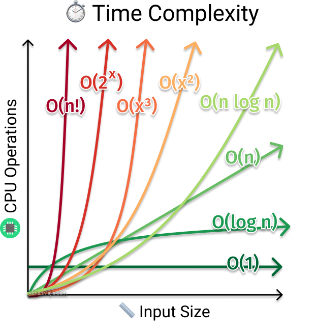
You don't need to know what O(log n) or O(n²) mean yet. The key insight is to see how drastically the lines diverge. An algorithm that follows the red O(n²) curve might be fine for an input of size 10, but it becomes completely impractical for an input of size 1,000,000 compared to an algorithm on the green O(n) curve.
Our goal in this module is to learn how to identify which curve an algorithm will follow.
3. A Tale of Two Computers: Efficiency Trumps Speed
Let's make this even more concrete. A common saying in computer science is: A faster algorithm on a slower computer will always beat a slower algorithm on a faster computer for a sufficiently large input.
The following reading provides an excellent example that translates the abstract "number of instructions" into real-world clock time.
[PDF] Introduction to Algorithms
These lecture notes from Northeastern University provide a table that quantifies the difference in performance. It's the perfect illustration of why a better algorithm is more important than a faster machine.
Start reading from the section 'Run time as Clock time' and continue through the table under 'Runtime, Clocktime, and Efficiency'. First, understand how the text connects the number of instructions (like n²) to actual seconds using the machine's speed (MIPS - millions of instructions per second). Next, carefully examine the table. Compare the runtime for an n² (quadratic) algorithm with an n (linear) one. For n=1000, the n² algorithm on the faster 'Intel i7 B' machine is faster (8.5µs) than the linear algorithm on the slower 'Intel i7 A' machine (20µs). But what happens when the input size n grows to 1,000,000? The linear algorithm is still incredibly fast (20µs on the slow machine), while the quadratic one would take a very, very long time (the table doesn't even show it, but it would be around 20,000 seconds, or over 5.5 hours!).
This table powerfully demonstrates the learning outcome for today. The choice of algorithm has a much greater impact on performance than the speed of the hardware, especially when dealing with large amounts of data. This is why companies and interviewers are so focused on algorithmic efficiency. As one of the resources mentioned, "we can buy more memory, but we can't buy more time."
Conclusion
In this lesson, we established the fundamental "why" behind algorithm analysis. It’s not just an academic exercise; it's a practical necessity for building software that can handle the massive scale of modern data.
Key Takeaways:
- Simply timing an algorithm is unreliable because results depend on the hardware and other external factors.
- The true test of an algorithm's efficiency is how its performance scales as the input size grows.
- Inefficient algorithms can become unusably slow for large inputs, even on the fastest computers.
- A more efficient algorithm on a slow machine will outperform a less efficient algorithm on a fast machine when the input is large enough.
We now have a clear motivation. We need a way to describe and compare how algorithms scale, independent of any specific computer.
Preview of the Next Lesson:
In the next lesson, we will learn the tool that computer scientists use to do exactly that. Your goal will be to define Big O notation and use it to express an algorithm's time complexity. This notation is the language we use to talk about efficiency, and it will be central to the rest of this course.