Counting Loop Operations

1. What Are We Counting? Primitive Operations

Before we can count, we need to know what to count. We're interested in the most basic steps a computer takes to execute a program. These are called primitive operations.

Think of them as the individual atoms of computation. Each one takes a small, roughly constant amount of time.

This first resource defines what a primitive operation is and gives clear examples.

As you can see, primitive operations include:

• Assigning a value to a variable (e.g., x = 5).
• Performing an arithmetic operation (e.g., a + b).
• Comparing two values (e.g., i < n).
• Accessing an element in a list by its index (e.g., my_list[0]).
• Returning a value from a function.

Our strategy will be to break down an algorithm into these primitive operations and count them up.

2. The Frequency Count Method

The technique we'll use is called the frequency count method. It's a straightforward idea: we'll look at each line of code, determine how many primitive operations it contains, and figure out how many times that line of code is executed.

The next video introduces this concept formally.

To summarize, the total number of operations is the sum of (cost of instruction) * (number of times it executes).

Let's apply this method to a simple loop.

3. Counting Operations in a Simple Loop

This is where things get interesting. Operations outside a loop run once, but operations inside a loop run many times. Let's analyze a function that finds the maximum value in a list of numbers.

def find_max(data):



    # Let n be the number of elements in 'data'
    # e.g., n = len(data)

    current_max = data[0]      # Line 1
    
    for i in range(1, n):      # Line 2
        if data[i] > current_max:  # Line 3
            current_max = data[i]  # Line 4
            
    return current_max         # Line 5

Let's break this down line-by-line. To make the counting explicit, we'll analyze the for loop as if it were a C-style loop, which is what happens under the hood. The following video gives an exceptionally clear and detailed walkthrough of this process.

Let's use the logic from the video to analyze our find_max function. Assume the input list data has n elements.

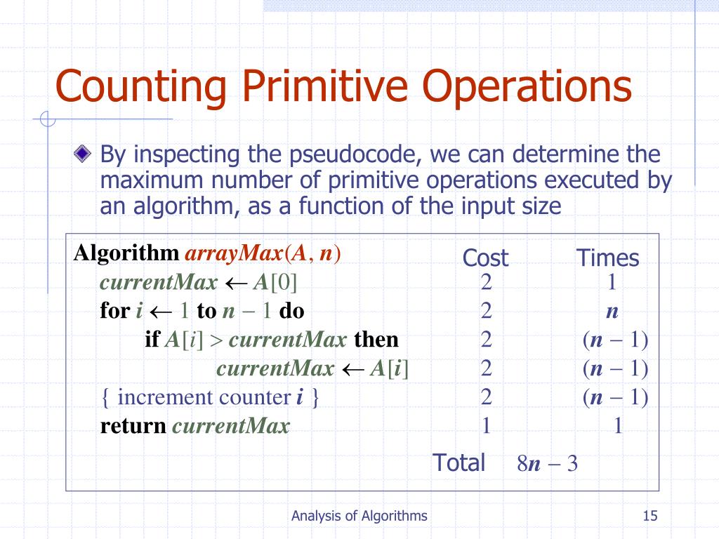
Let's trace the execution based on the image's logic:

• current_max = data[0]: This line runs once. It involves one list access and one assignment, so let's say it costs 2 operations.
  • Total: 2 ops
• The for loop: The loop runs from i = 1 to n-1. This means the loop body will execute n-1 times.
  • The loop control itself involves initializing i, comparing i against n at each step, and incrementing i. Based on the video, the comparison will happen n times (for i=1, 2, ..., n-1, and one final time to exit the loop). The increment will happen n-1 times.
• if data[i] > current_max: This line is inside the loop, so it executes n-1 times. It involves one list access and one comparison.
  • Cost per iteration: 2 ops. Total: 2 * (n-1) ops
• current_max = data[i]: This line is tricky. It only runs when we find a new maximum. In the worst case (a sorted list), it runs every single time, so n-1 times. In the best case (a reverse-sorted list), it never runs. For analysis, we usually focus on the worst case. It involves one list access and one assignment.
  • Worst-case cost per iteration: 2 ops. Total: 2 * (n-1) ops
• return current_max: This runs once.
  • Total: 1 op

Adding it all up (and simplifying the loop control costs for now), a rough worst-case count is 2 + (n-1)*2 + (n-1)*2 + 1, which simplifies to 2 + 4(n-1) + 1 = 4n - 4 + 3 = 4n - 1.

Don't worry about getting the exact count. The key takeaway is that the total number of operations is a function of n, like 4n - 1.

4. Counting Operations in Nested Loops

What happens when you put a loop inside another loop?

# Let n be a positive integer
count = 0
for i in range(n):      # Outer loop
    for j in range(n):  # Inner loop
        count = count + 1

The logic is multiplicative. The outer loop runs n times. For each of those n iterations, the inner loop also runs n times.

So, the statement count = count + 1 will execute n * n = n² times.

The following video demonstrates this with examples of matrix addition (two nested loops) and matrix multiplication (three nested loops).

A More Precise Count for Nested Loops

Not all nested loops are as simple as n * n. Consider this code, which checks for duplicate elements in a list.

def has_duplicates(items):
    n = len(items)
    for i in range(n):
        for j in range(i + 1, n):



            # This comparison is our basic operation
            if items[i] == items[j]:
                return True
    return False

Let's count how many times the comparison items[i] == items[j] runs in the worst case (no duplicates).

• When i is 0, j goes from 1 to n-1. ( n-1 comparisons)
• When i is 1, j goes from 2 to n-1. ( n-2 comparisons)
• When i is 2, j goes from 3 to n-1. ( n-3 comparisons)
• ...
• When i is n-2, j goes from n-1 to n-1. (1 comparison)
• When i is n-1, the inner loop doesn't run at all. (0 comparisons)

The total number of comparisons is the sum: (n-1) + (n-2) + ... + 1.
This is a classic arithmetic series. The sum is given by the formula k(k+1)/2 where k = n-1.
So, the total is (n-1)(n-1+1)/2 = (n-1)n / 2 = (n² - n) / 2.

Again, notice that the result is an expression involving n². This is typical for algorithms with two nested loops. For more details on this kind of analysis, you can refer to the "Element Uniqueness Problem" example in the document from Jsums.edu (LINK, section 5). Given your math background, you might find the summation notation used there quite natural.

Conclusion

In this lesson, you learned the hands-on process of analyzing an algorithm by counting its primitive operations. This gives us a concrete, machine-independent number that represents the work an algorithm does.

Key Takeaways:

• Primitive operations are the basic steps of a program (assignment, arithmetic, comparison).
• The frequency count method involves summing up the number of times each operation is executed.
• For a simple loop that runs n times, the total number of operations will be a linear function of n (e.g., 4n - 1).
• For a nested loop where both loops run n times, the total operations will be a quadratic function of n (e.g., (n² - n) / 2).

You might already be thinking that calculating the exact count, like 4n - 1 or (n² - n) / 2, is tedious and a bit messy. You're right! What really matters is not the exact number, but the dominant term (4n or n²) that determines how the runtime grows.

Preview of the Next Lesson:
In our next lesson, we will introduce a powerful tool to formalize this simplification. Your learning outcome will be to define Big O notation and use it to express an algorithm's time complexity. Big O notation is the standard language for talking about algorithm efficiency, allowing us to ignore the small details and focus on the big picture of how an algorithm scales.