Comparing Algorithm Efficiency with Big O

Why Comparison Matters: Scalability

The core reason we use Big O notation is to understand how an algorithm scales. An inefficient algorithm might work perfectly fine for an input of 10 items, but it could become unusably slow for 10 million items. Big O helps us predict this behavior without having to run the code on massive datasets.

Let's look at a chart that visualizes this.

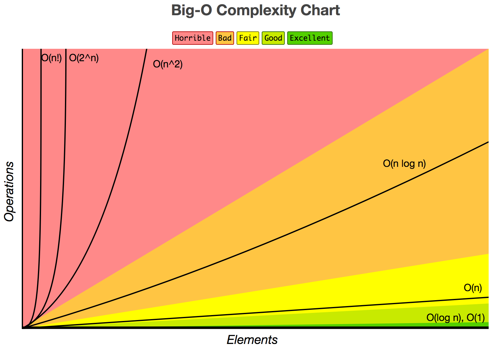
As you can see, an algorithm with O(n²) complexity becomes very slow, very quickly. In contrast, an O(log n) algorithm's runtime barely increases, even for huge inputs. This is the essence of scalability.

Case Study 1: O(n) vs. O(1)

Let's consider a simple problem: calculating the sum of all integers from 1 to n.

There are at least two ways to solve this.

Algorithm A: The Looping Sum
The most straightforward way is to loop from 1 to n and add each number to a running total.

def sum_with_loop(n):
    total = 0



    # This loop runs 'n' times
    for i in range(1, n + 1):
        total += i
    return total

Based on the previous lesson, you can see this function has a single loop that runs n times. This is a classic O(n) or linear time complexity.

Algorithm B: The Mathematical Formula
A more clever approach uses a mathematical formula you might have seen before, often attributed to Gauss.

def sum_with_formula(n):



    # This involves a few constant-time operations
    return (n * (n + 1)) // 2

This function performs one multiplication, one addition, and one division, regardless of the value of n. Its complexity is O(1) or constant time.

The following short video demonstrates this exact comparison.

Comparison:

• sum_with_loop: O(n)
• sum_with_formula: O(1)

For n = 1,000,000, the loop-based function performs roughly one million operations. The formula-based function performs just three. The O(1) algorithm is vastly superior because its performance is independent of the input size. It scales perfectly.

Case Study 2: O(n) vs. O(log n)

Now let's tackle another common problem: searching for an element in a list.

Algorithm A: Linear Search
This approach iterates through each item in the list until it finds the target. It works on any list, sorted or not. In the worst case (the item is at the end or not present), it must check all n elements.

• Complexity: O(n)

Algorithm B: Binary Search
This "divide and conquer" algorithm is much more efficient, but it comes with a critical requirement: the list must be sorted. It works by repeatedly checking the middle element and discarding the half of the list where the target cannot be.

• Complexity: O(log n)

The image below shows the difference in their search process.

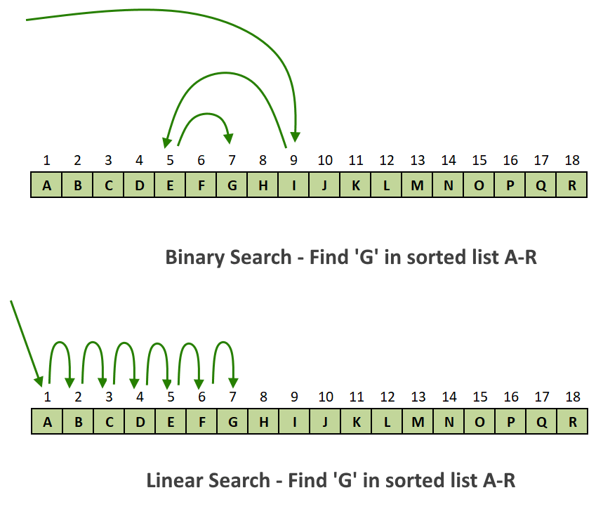
To understand the analysis in more detail, let's look at a resource that breaks down the operation counts for both algorithms.

Comparison:

• Linear Search: O(n)
• Binary Search: O(log n)

As the table on slide 38 shows, the difference is staggering. For a list of 1,000,000 items:

• Linear search takes, on average, around 750,000 comparisons.
• Binary search takes, in the worst case, only 20 comparisons.

This is a powerful demonstration of why an O(log n) algorithm is highly desirable for large datasets. The trade-off is the need to have the data sorted beforehand.

Case Study 3: O(n) vs. O(n²)

Let's revisit two algorithms from a previous lesson.

• find_max (finding the largest element): Involves one loop through the list. This is O(n).
• has_duplicates (checking for duplicate elements): Involves a nested loop comparing every element to every other element. This is O(n²).

The following video visually contrasts the growth rates of linear (O(n)) and quadratic (O(n²)).

Comparison:

• find_max: O(n)
• has_duplicates: O(n²)

As the video explains, even if the O(n²) algorithm is faster for a tiny input (e.g., n=5) due to having fewer instructions overall (lower constant factors), the O(n) algorithm will always win as n gets larger. The shape of the growth curve is what matters in the long run.

General Rules for Comparison

We can generalize these comparisons into a hierarchy of efficiency. For large inputs, an algorithm with a lower growth rate is always better.

O(1) < O(log n) < O(n) < O(n log n) < O(n²) < O(2ⁿ) < O(n!)
Excellent <---------- Good ----------> Bad <----- Horrible

The following reading explains the rules for determining which functions grow faster.

A Note of Caution: When Big O Can Be Misleading

While Big O is our primary tool for comparison, a purely mathematical analysis can sometimes miss real-world nuances. It's important to remember that Big O describes the asymptotic behavior (as n approaches infinity) and ignores constant factors.

For example, consider two famous sorting algorithms:

• Merge Sort: Has a worst-case and average-case complexity of O(n log n).
• Quicksort: Has an average-case of O(n log n) but a worst-case of O(n²).

Based on a worst-case analysis, Merge Sort seems like the clear winner. However, in practice, Quicksort is often faster because its average-case performance has better "constant factors"—it's simply a more efficient set of operations, on average.

This next reading explores this important caveat.

This doesn't mean Big O is wrong; it just means it's a model. For interviews and general algorithm design, comparing algorithms by their worst-case Big O complexity is the standard and correct approach. But having this deeper understanding of the nuances will set you apart.

Conclusion

You've made a huge leap today, moving from just identifying complexity to actively using it to compare and evaluate algorithms. This is one of the most fundamental skills in computer science.

Key Takeaways:

• Big O notation allows us to compare how algorithms scale as input size (n) grows.
• An algorithm with a lower order of growth is generally more efficient for large inputs (e.g., O(log n) is better than O(n)).
• When comparing algorithms, we often look for solutions with better Big O complexity to solve the same problem.
• This choice can involve trade-offs, such as binary search requiring a pre-sorted list.
• While worst-case Big O is the standard for comparison, real-world performance can also be influenced by average-case behavior and constant factors.

Preview of the Next Lesson:
We briefly touched on the idea of best, average, and worst-case performance in this lesson. In our next session, we will formalize this. You will learn to explain the difference between best-case, worst-case, and average-case complexity, giving you an even more precise language to discuss algorithm efficiency.