Big O Notation: Common Time Complexities

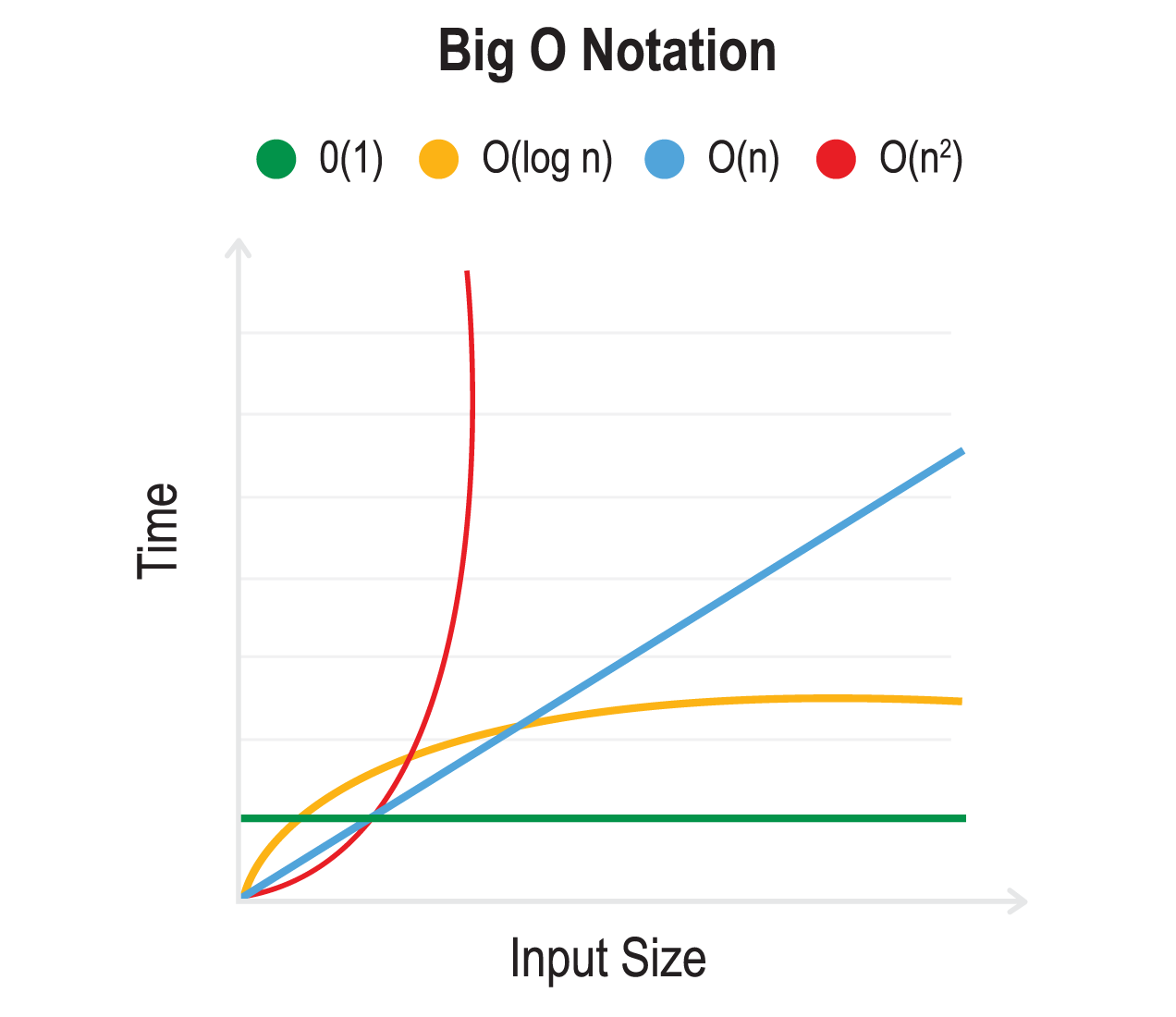
1. O(1) — Constant Time

An algorithm has constant time complexity if its execution time does not change, regardless of the size of the input. It performs a fixed number of operations.

Common Patterns:

• A mathematical calculation (e.g., 2 + 2).
• Assigning a value to a variable.
• Accessing an element in a data structure by its index or key (like a Python list or dictionary).

The following video provides a clear explanation and some great examples.

As the video explained, operations are O(1) if they take the same amount of time regardless of how much data is being stored.

Here's a simple Python example. This function retrieves the first and last elements of a list and returns their sum.

def get_first_and_last_sum(numbers):



    # This assumes the list is not empty
    first_element = numbers[0]    # O(1) - Indexing is constant time
    last_element = numbers[-1]   # O(1) - Indexing is constant time
    return first_element + last_element # O(1) - Arithmetic is constant time

No matter if the numbers list has 10 elements or 10 million elements, this function performs the same three basic operations. Its complexity is constant, which we denote as O(1).

2. O(n) — Linear Time

An algorithm has linear time complexity if its execution time grows in direct proportion to the size of the input, n. If you double the input size, the runtime will also roughly double.

Common Pattern:

• A single for or while loop that iterates through all n elements of a collection.

Let's return to the NeetCode video for an explanation of linear time.

Here is a Python function that finds the largest number in a list. We analyzed this in a previous lesson by counting its operations. Now, we can identify its complexity simply by recognizing the pattern.

def find_max(numbers):



    # This assumes the list is not empty
    max_value = numbers[0]  # O(1)
    



    # This loop runs 'n' times, where n is len(numbers)
    for number in numbers:    # O(n)
        if number > max_value:
            max_value = number
            
    return max_value

The dominant part of this function is the for loop, which runs n times. The work inside the loop is constant (O(1)). Therefore, the overall complexity is O(n).

3. O(n²) — Quadratic Time

An algorithm has quadratic time complexity if its runtime grows proportionally to the square of the input size. If you double the input size, the runtime will roughly quadruple (2² = 4).

Common Pattern:

• A nested loop, where both the outer and inner loops iterate through the n elements of a collection. This results in n * n = n² operations.

This pattern is common in algorithms that need to compare every element in a collection to every other element.

Let's look at a concrete code example. This function checks if a list contains any duplicate values by comparing every pair of elements.

def has_duplicates(items):
    n = len(items)
    for i in range(n):        # This outer loop runs n times
        for j in range(n):    # This inner loop runs n times for each outer iteration
            if i != j and items[i] == items[j]:
                return True   # Found a duplicate
    return False

Because the inner loop runs n times for each of the n iterations of the outer loop, the total number of comparisons is n * n = n². This makes the algorithm's complexity O(n²). As you can see from the graph at the start of the lesson, this gets slow very quickly!

4. O(log n) — Logarithmic Time

Logarithmic time complexity is highly efficient. The runtime grows very slowly, even for very large inputs. The core idea is that the algorithm reduces the size of the problem by a constant factor (usually half) at each step.

Given your math background, you'll recognize the definition of a logarithm. For our purposes, log₂(n) answers the question: "How many times can I cut n in half until I get down to 1?"

Common Patterns:

• Algorithms that repeatedly divide the search space, like binary search on a sorted array.
• A loop where the counter variable is multiplied or divided by a constant at each step.

This next video provides an excellent, foundational explanation of logarithms in the context of computer science, and then shows how it relates to code.

As the video demonstrated, any process that consistently reduces the problem size by a constant factor is logarithmic. Here's a simple iterative example in Python:

def logarithmic_function(n):



    # This assumes n is a positive number
    i = n
    while i > 1:
        print(i)
        i = i / 2  # The work is halved at each step

If n were 16, the loop would run with i being 16, 8, 4, and 2. It only takes 4 steps. If n were 1,024, it would only take 10 steps. The number of steps is log₂(n). We simplify this to O(log n).

Summary and Practice

Let's consolidate what you've learned.

Now, try to identify the time complexity of the following Python functions based on these patterns.

Practice 1:

def check_first_item(items):
    if len(items) > 0:
        if items[0] == "hello":
            return True
    return False

Practice 2:

def print_all_numbers(numbers):
    for n in numbers:
        print(n)

Practice 3:

def count_until_half(n):
    count = 0
    i = n
    while i > 1:
        count += 1
        i = i // 2 # Integer division
    return count

Practice 4:

def create_pairs(items):
    pairs = []
    for item1 in items:
        for item2 in items:
            pairs.append((item1, item2))
    return pairs

Conclusion

Great job! You are now equipped to quickly analyze the efficiency of a wide range of simple algorithms by recognizing their underlying structure. This skill is fundamental to writing better code and is a frequent topic in technical interviews.

Key Takeaways:

• O(1) (Constant): A fixed number of operations.
• O(n) (Linear): A single loop iterating through n items.
• O(n²) (Quadratic): Nested loops iterating through n items.
• O(log n) (Logarithmic): A process that repeatedly halves the input.

Preview of the Next Lesson:
Now that you can identify the Big O complexity of different algorithms, the next logical step is to use that information. In the next lesson, you will learn how to compare two algorithms for the same problem using Big O analysis. This will help you understand the practical trade-offs and make informed decisions about which approach is better suited for a given task.