Binary Search: Implementation and Complexity Analysis

1. The Core Idea: Divide and Conquer

Instead of checking every single element, what if we could eliminate half of the remaining elements with a single check? This is the central idea of binary search.

Imagine you're looking for a word in a physical dictionary. You don't start at "A" and read every word. You open it somewhere in the middle. If your word comes alphabetically before the words on that page, you know your word is in the first half of the dictionary. If it comes after, you know it's in the second half. You've just eliminated half the dictionary in one step. You can then repeat this process on the remaining half.

This strategy has a name: divide and conquer. Let's explore this with a non-technical analogy.

As the article explains, you repeatedly divide the problem space (the time the bike could have been stolen, or the part of the list where an element could be) in two.

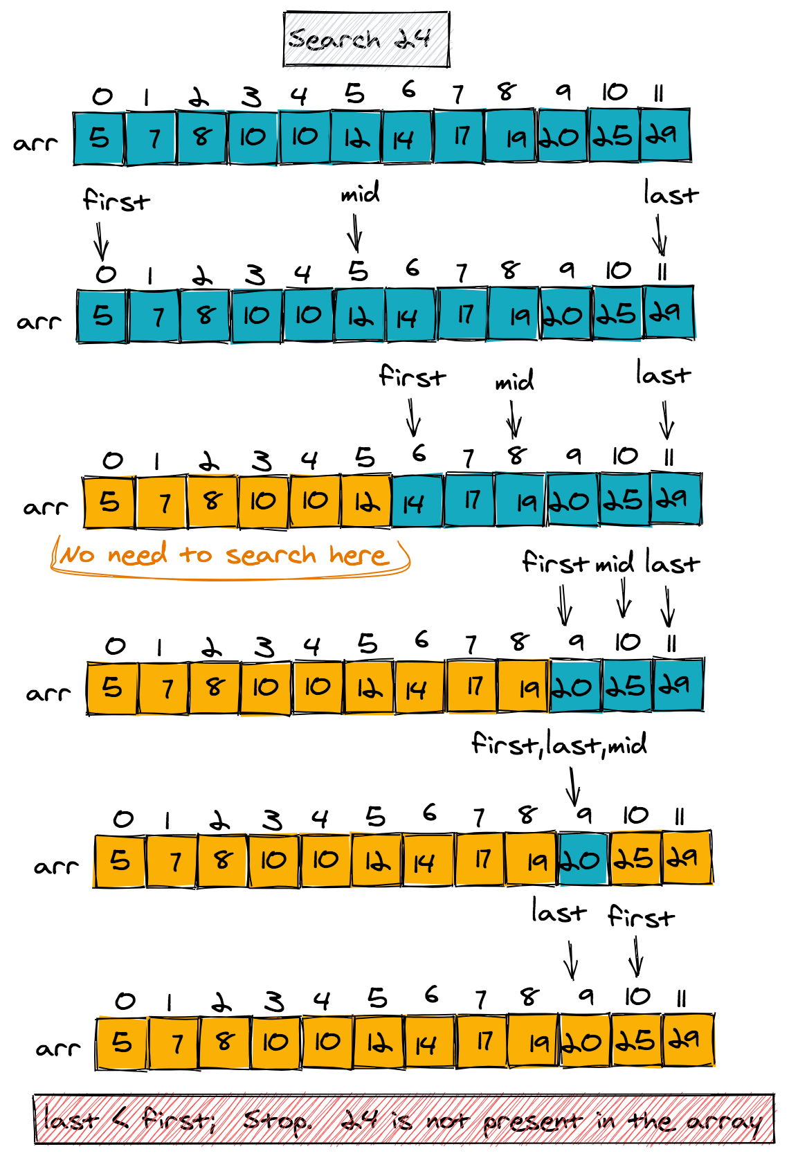
Let's see how this applies to a sorted list of numbers. The "middle of the dictionary" becomes the middle element of our list.

2. Implementing Binary Search in Python

Now that we have the intuition, let's translate this "divide and conquer" logic into Python code. We will implement an iterative version of binary search using a while loop.

We'll need to keep track of three things:

1. A low pointer to mark the beginning of our current search space.
2. A high pointer to mark the end.
3. A mid pointer that we calculate in each step.

This video provides an excellent walkthrough of the core concept and a clear, step-by-step implementation.

Let's review the code from the video. It's a standard and effective implementation of binary search.

def binary_search(sequence, item):



    # Set the boundaries of the search space
    begin_index = 0
    end_index = len(sequence) - 1




    # Loop as long as the search space is valid
    while begin_index <= end_index:



        # Calculate the midpoint index (using floor division //)
        midpoint = begin_index + (end_index - begin_index) // 2
        midpoint_value = sequence[midpoint]




        # Compare the midpoint value with the item we're looking for
        if midpoint_value == item:



            # Found it! Return the index.
            return midpoint
        elif item < midpoint_value:



            # The item must be in the left half
            end_index = midpoint - 1
        else:



            # The item must be in the right half
            begin_index = midpoint + 1
    



    # If the loop finishes, the item was not in the sequence
    return None




# --- Let's test it! ---
sorted_list = [2, 5, 8, 12, 16, 23, 38, 56, 72, 91]




# Case 1: Target is in the list
target1 = 23
result1 = binary_search(sorted_list, target1)
print(f"Searching for {target1}: Found at index {result1}")




# Case 2: Target is not in the list
target2 = 50
result2 = binary_search(sorted_list, target2)
if result2 is not None:
    print(f"Searching for {target2}: Found at index {result2}")
else:
    print(f"Searching for {target2}: Not found in the list.")

Your Turn: Practice with the Code

1. Copy the binary_search function and the test cases into a Python file.
2. Run the code to confirm you get the same output.
3. Add test cases to search for:
   • The very first element (2).
   • The very last element (91).
   • An element smaller than any in the list (e.g., 1).
4. Before running your new tests, trace the values of begin_index, end_index, and midpoint on paper for one of the cases. This will solidify your understanding of how the search space shrinks.

3. Analyzing Time Complexity: What is O(log n)?

We know binary search is fast, but how fast? Its time complexity is O(log n) (read "O of log n"). To understand this, we first need a clear, intuitive grasp of what a logarithm represents in computer science.

Your math background with exponents will be very helpful here. A logarithm is the inverse of an exponent. The expression ${\log }_2(n)$ asks the question: "How many times must I multiply 2 by itself to get n?"

In algorithms, we can flip this question around: "Starting with n, how many times can I divide it by 2 until I get down to 1?" This is exactly what binary search does to its search space.

This first video gives a great explanation.

Now, let's connect that concept directly to our binary search algorithm.

To formalize this, consider an array of n elements.

• After 1 comparison, the search space is at most n / 2.
• After 2 comparisons, it's at most n / 4.
• After k comparisons, it's at most n / 2^k.

The search ends when the search space has size 1. So, in the worst case, we are looking for the number of steps, k, where n / 2^k = 1. Solving for k gives us n = 2^k, which means k = log₂(n). This is why the time complexity is O(log n).

This article section provides a concise summary of this mathematical reasoning.

The difference between O(n) and O(log n) is not just a small improvement; it's monumental for large inputs.

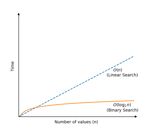
For a list with a million items, linear search might take a million steps. Binary search would take only about 20 steps (${\log }_2(1,000,000)\approx 19.9$). This is the power of a better algorithm.

Conclusion

Fantastic work today! You've tackled one of the most important and elegant algorithms in computer science.

Key Takeaways:

• Binary search operates on sorted data only.
• It uses a divide and conquer approach, repeatedly halving the search space with each comparison.
• The iterative implementation uses low, high, and mid pointers to manage the search space within a while loop.
• The time complexity is O(log n), which is exceptionally fast because the number of operations grows very slowly as the input size n increases.

Preview of the Next Lesson:
We've now seen how efficient searching can be if a list is sorted. But what if our data isn't sorted to begin with? In the next lesson, we'll shift our focus from searching to sorting and implement our first sorting algorithm, insertion sort. We'll see how it works and analyze its O(n²) time complexity.