Rolling Without Slipping: Constraint Application

1. The Classic Case: Rolling on a Stationary Incline

The most fundamental application of the rolling constraint is analyzing an object rolling down an inclined plane. Here, we must combine the kinematic constraint with dynamic principles (Newton's Second Law for translation and rotation).

To see a masterclass in this derivation and its surprising consequences, let's turn to a lecture by Prof. Walter Lewin.

Let's formalize the steps from the video. For an object with mass $M$, radius $R$, and moment of inertia $I_{CM}$ rolling down a plane inclined at an angle $\beta$:

1. Linear Dynamics (Newton's 2nd Law): The net force along the incline is the component of gravity minus the static friction force $F_f$.
   $Mg\sin \beta -F_f=M{a}_{CM}$

2. Rotational Dynamics (Torque Equation): The only force creating a torque about the center of mass is friction.
   ${\tau }_{CM}=R{F}_f=I_{CM}\alpha$

3. Kinematic Constraint: The condition for rolling without slipping connects linear and angular acceleration.
   $a_{CM}=\alpha R$

You now have a system of three equations with three unknowns ($a_{CM}$, $\alpha$, and $F_f$). The key insight is that the kinematic constraint is the bridge that allows you to solve this system. By substituting $\alpha =a_{CM}/R$ and $F_f=I_{CM}{a}_{CM}/R^2$ into the force equation, you can solve for $a_{CM}$:

$a_{CM}=\frac{g\sin \beta }{1+I_{CM}/(M{R}^2)}$

As Prof. Lewin demonstrates, for a given shape (which determines the ratio $I_{CM}/(M{R}^2)$), the acceleration is independent of mass and radius. This is a non-intuitive result that follows directly from a rigorous application of our constraint.

2. Upgrading the Challenge: Rolling on a Moving Surface

What happens when the surface itself is in motion? The fundamental principle, ${\vec{v}}_{\text{body at contact}}={\vec{v}}_{\text{surface at contact}}$, remains unchanged. However, the right-hand side of the equation is no longer zero.

The following resource provides a formal vector-based treatment for this exact scenario.

The derivation in the paper shows that the velocity of the center of mass $G$ is given by:
${\dot{\vec{r}}}_G={\dot{\vec{r}}}_{CS}+{\vec{\omega }}_B\times {\vec{r}}_{GCB}$
This is a direct application of the principles we've discussed. Let's apply this to a challenging problem.

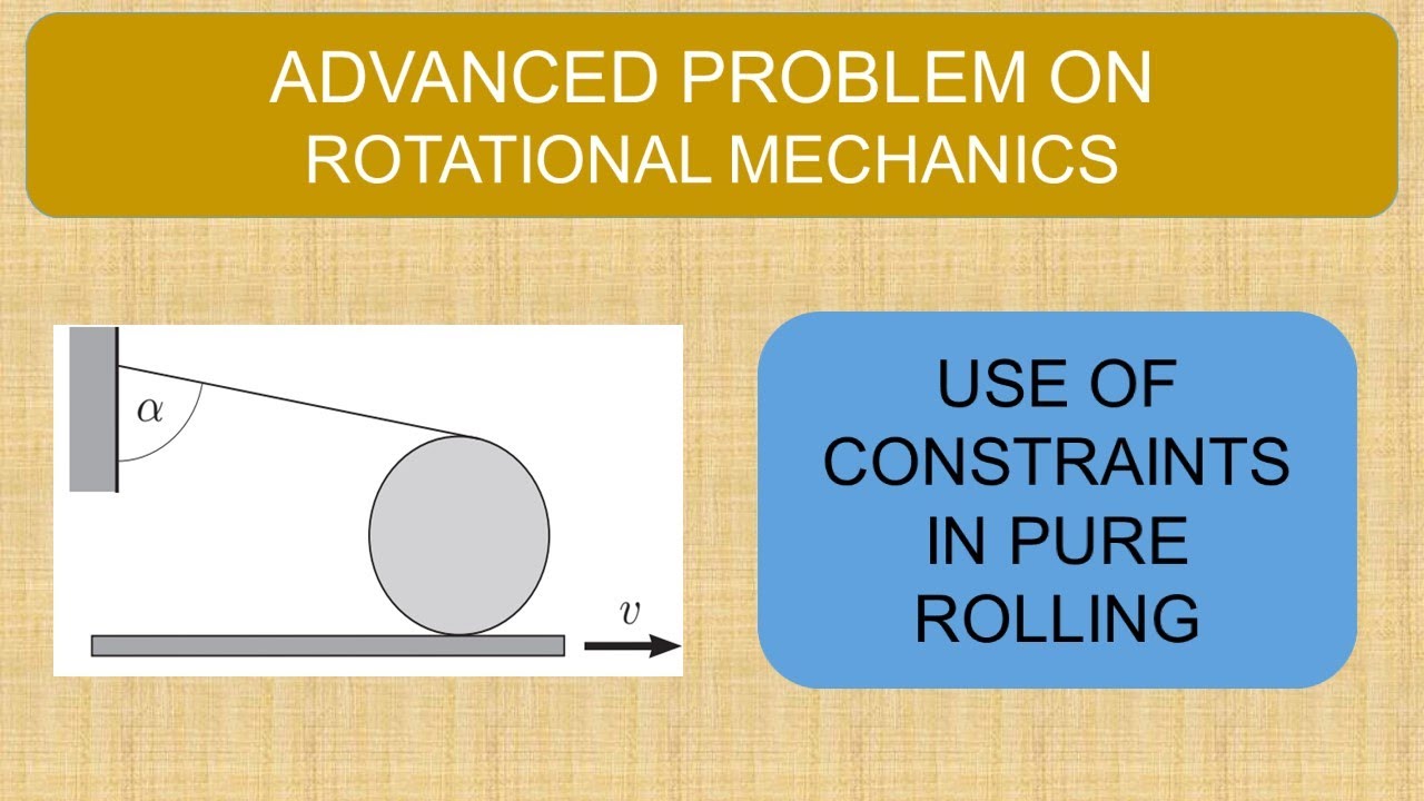
Problem Analysis:

We have two constraints acting on the cylinder:

1. Rolling without slipping on the plank.
2. The inextensible string.

Let's assume the cylinder's center moves to the right with velocity $v_c$ and rotates clockwise with angular speed $\omega$. In vector terms: ${\vec{v}}_c=v_c\hat{i}$ and $\vec{\omega }=-\omega \hat{k}$. The plank's velocity is ${\vec{v}}_p=v_p\hat{i}$.

Applying the Rolling Constraint:
The contact is at the bottom of the cylinder ($P_{bot}$).
${\vec{v}}_{P_{bot}}={\vec{v}}_p$
The velocity of $P_{bot}$ on the cylinder is ${\vec{v}}_c+\vec{\omega }\times {\vec{r}}_{P_{bot}/c}$. The position vector from the center to the bottom is ${\vec{r}}_{P_{bot}/c}=-R\hat{j}$.
$v_c\hat{i}+(-\omega \hat{k})\times (-R\hat{j})=v_c\hat{i}-\omega R\hat{i}=(v_c-\omega R)\hat{i}$
Equating this to the plank's velocity:
$(v_c-\omega R)\hat{i}=v_p\hat{i}⟹v_c-\omega R=v_p\text{(Eq. 1)}$

Applying the String Constraint:
The string is attached to the top of the cylinder ($P_{top}$). The velocity component of this point along the string must be zero (since the wall is fixed and the string is inextensible).
First, find the velocity of $P_{top}$. The position vector is ${\vec{r}}_{P_{top}/c}=R\hat{j}$.
${\vec{v}}_{P_{top}}={\vec{v}}_c+\vec{\omega }\times {\vec{r}}_{P_{top}/c}=v_c\hat{i}+(-\omega \hat{k})\times (R\hat{j})=(v_c+\omega R)\hat{i}$
The string direction vector $\hat{s}$ points from $P_{top}$ to the wall. From the diagram, it's left and up. The angle with the vertical is $\alpha$, so the angle with the negative x-axis is $90^{\circ }-\alpha$.
$\hat{s}=-\cos (90^{\circ }-\alpha )\hat{i}+\sin (90^{\circ }-\alpha )\hat{j}=-\sin \alpha \hat{i}+\cos \alpha \hat{j}$
The constraint is ${\vec{v}}_{P_{top}}\cdot \hat{s}=0$.
$((v_c+\omega R)\hat{i})\cdot (-\sin \alpha \hat{i}+\cos \alpha \hat{j})=0$
$-(v_c+\omega R)\sin \alpha =0$
Since $\alpha \ne 0$, we must have:
$v_c+\omega R=0⟹v_c=-\omega R\text{(Eq. 2)}$
This implies the cylinder actually moves to the left ($v_c<0$) and rotates counter-clockwise ($\omega <0$), or vice versa. Let's stick with the math.

Solving the System:
From (2), $\omega =-v_c/R$. Substitute this into (1):
$v_c-(-v_c/R)R=v_p$
$v_c+v_c=v_p⟹2v_c=v_p⟹{\mathbf{v}}_{\mathbf{c}}=\frac{{\mathbf{v}}_{\mathbf{p}}}{2}$
The center of the cylinder moves to the right at half the speed of the plank. Its angular velocity is $\omega =-v_c/R=-v_p/(2R)$, indicating counter-clockwise rotation, which makes physical sense for this setup.

3. Advanced Application: A JEE Advanced Problem

To meet the demands of advanced competitive exams, you must be able to apply the no-slip condition in more abstract and complex geometries, such as systems with multiple simultaneous rotations.

The following video breaks down a JEE Advanced problem that is a perfect example of this complexity. It involves two discs fixed by a rod, rolling on a surface while the entire assembly also rotates.

The crucial step in this problem is recognizing that the velocity of the contact point P is the vector sum of velocities due to two separate rotations:

1. Rotation of the disc about its own center, with angular speed $\omega$.
2. Rotation of the entire assembly about a vertical axis (the z-axis), with angular speed ${\omega }_z$.

The no-slip condition, ${\vec{v}}_P=0$, is then written as a vector equation:
${\vec{v}}_{P,\text{rot 1}}+{\vec{v}}_{P,\text{rot 2}}=0$
By calculating the magnitudes and noting the opposing directions of these two velocity components, the problem becomes solvable. This method of decomposing motion and applying the constraint is a powerful strategy for advanced problems.

For another perspective on advanced problem-solving, the Olympiad-level handout below contains numerous challenging examples. "Example 4: MPPP 49" is particularly instructive as it shows a case where one must not only apply the constraint but also check the physical validity of the result (i.e., ensuring a string's tension is non-negative).

Conclusion

Today we have transitioned from the abstract derivation of the rolling constraint to its concrete application in a variety of physical contexts. The complexity can increase, but the core principle remains constant.

Key Takeaways:

• The rolling-without-slipping constraint, ${\vec{v}}_{\text{body at contact}}={\vec{v}}_{\text{surface at contact}}$, is the fundamental tool for solving rolling problems.
• For stationary surfaces, this constraint is often used with Newton's laws to solve for acceleration and forces like friction.
• For moving surfaces, the velocity of the surface provides a non-zero term in the constraint equation, which must be correctly accounted for.
• In complex systems with multiple rotations, the velocity of the contact point is the vector sum of velocities from each rotation. The no-slip constraint applies to this resultant velocity.
• Advanced problem solving requires not only applying the constraint correctly but also verifying that the results are physically plausible (e.g., tension in a string cannot be negative).

Preview of the Next Lesson:

Having explored various types of constraints, we will now shift our focus to a different class of advanced kinematics problems. In our next lesson, we will solve complex problems involving minimum or maximum time/distance by applying calculus optimization to kinematic equations. This will involve setting up kinematic functions and using derivatives to find their extrema, a technique frequently required in Olympiad-level questions.