1D Relative Velocity: Chases, Meetings, and Separation

Hello! Welcome back.

In our last lesson, we undertook a significant theoretical task: deriving the general vector equations that transform position, velocity, and acceleration between arbitrarily moving and rotating reference frames. We established that the acceleration of a particle $P$ in a fixed frame $S$ is related to its acceleration in a moving frame $S^{'}$ by:
$a_{P} = a_{S^{'}} + a_{P / S^{'}} + α_{S^{'}} \times r_{P / S^{'}} + Ω \times (Ω \times r_{P / S^{'}}) + 2 (Ω \times v_{P / S^{'}})$
This equation, containing terms for frame acceleration, relative acceleration, tangential, centripetal, and Coriolis effects, is the complete kinematic description.

Today, we will begin to put this powerful framework to practical use. Our learning outcome is to apply relative velocity concepts to solve 1D problems involving chases, meetings, and separation. We will see how the general vector equations simplify dramatically in one dimension and provide an elegant and systematic method for solving problems that might otherwise seem complex.

1. Specializing the General Equations for 1D Motion

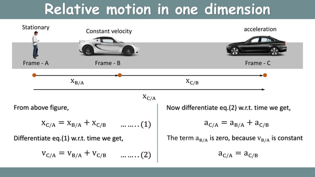
Let's consider two objects, A and B, moving along a single straight line (the x-axis). We can analyze the motion of A from the perspective of B. In this context, the "lab" frame is our fixed frame $S$ , and the reference frame attached to object B is our moving frame $S^{'}$ .

Since the motion is purely translational along a line, there is no rotation. This gives us a crucial simplification:

Angular velocity $Ω = 0$
Angular acceleration $α_{S^{'}} = 0$

Substituting these into our general velocity and acceleration equations from the last lesson makes most of the terms vanish.

The general velocity equation:
$v_{P / S} = v_{S^{'} / S} + v_{P / S^{'}} + Ω \times r_{P / S^{'}}$
...simplifies to:
$v_{P / S} = v_{S^{'} / S} + v_{P / S^{'}}$

And the general acceleration equation:
$a_{P / S} = a_{S^{'} / S} + a_{P / S^{'}} + α_{S^{'}} \times r_{P / S^{'}} + Ω \times (Ω \times r_{P / S^{'}}) + 2 (Ω \times v_{P / S^{'}})$
...simplifies to:
$a_{P / S} = a_{S^{'} / S} + a_{P / S^{'}}$

Translating this into the notation of objects A and B, where we observe A from B's frame:

Particle $P$ is object A.
Moving frame $S^{'}$ is object B.
Fixed frame $S$ is the ground (or lab frame).

The equations become:

Relative Velocity: $v_{A / ground} = v_{B / ground} + v_{A / B}$
Relative Acceleration: $a_{A / ground} = a_{B / ground} + a_{A / B}$

Rearranging these gives the expressions for relative velocity and acceleration, which are the quantities an observer on B would measure for A:
$v_{A / B} = v_{A / ground} - v_{B / ground}$
$a_{A / B} = a_{A / ground} - a_{B / ground}$

In one dimension, these vector equations become simple scalar subtractions, paying attention to signs.

Relative Motion in One Dimension with Derivations — This diagram illustrates the fundamental equations for relative position, velocity, and acceleration in one dimension. Frame A is the stationary ground, Frame B is a car moving at constant velocity relative to A, and Frame C is another object accelerating relative to B. The equations show how the measurements in Frame A (e.g., $V_{C/A}$) are related to measurements in Frame B (e.g., $V_{C/B}$) and the motion of Frame B itself ($V_{B/A}$).

2. The Core Principle: Simplifying Motion

The "why" behind using this framework is that it can transform a two-body problem into a one-body problem.

Consider the motion of object A relative to object B. The equation of motion for A as seen by B is:
$x_{A / B} (t) = x_{A / B} (0) + v_{A / B} (0) t + \frac{1}{2} a_{A / B} t^{2}$
This is valid if and only if the relative acceleration, $a_{A / B}$ , is constant. This is a very common scenario. For example, if two cars, A and B, have different constant accelerations $a_{A}$ and $a_{B}$ , their relative acceleration $a_{A / B} = a_{A} - a_{B}$ is also a constant. The problem of analyzing A's motion relative to B becomes a standard constant-acceleration kinematics problem.

Let's apply this principle to some classic problem types.

3. Application 1: Chase and Overtaking Problems

These problems involve one object catching up to another. The key questions are typically "when?" and "where?" do they meet, or "how fast?" is one going when it catches the other.

Let's analyze a classic chase scenario.

Chapter 2 - Kinematics in 1-D

The following problem from David Morin's 'Introduction to Classical Mechanics' describes a police motorcycle chasing a car. It's a perfect first example.

Please read Multiple-choice Question 2.7. First, try to solve it on your own. Then, review the provided solution, which uses both a graphical and an algebraic method.

Now, let's re-examine this problem from a rigorous relative motion perspective.

Problem Setup:

Car (C): Constant velocity $v_{C} = v_{0}$ . Constant acceleration $a_{C} = 0$ .
Motorcycle (M): Starts from rest, $v_{M, 0} = 0$ . Constant acceleration $a_{M} = a$ .
They start at the same position, so their initial relative position is $x_{M / C} (0) = 0$ .

Analysis in the Car's Reference Frame:
In the reference frame of the car, the car is stationary. What does the motorcycle's motion look like?

Relative Initial Velocity: $v_{M / C} (0) = v_{M} (0) - v_{C} (0) = 0 - v_{0} = - v_{0}$ .
(Initially, the motorcycle appears to move backward from the car's perspective.)
Relative Acceleration: $a_{M / C} = a_{M} - a_{C} = a - 0 = a$ .
(The car sees the motorcycle accelerating towards it with acceleration $a$ .)

The motorcycle starts at $x_{M / C} (0) = 0$ with velocity $- v_{0}$ and acceleration $a$ . It "catches up" to the car when its position relative to the car is again zero, i.e., $x_{M / C} (t) = 0$ .

The equation for relative position is:
$x_{M / C} (t) = x_{M / C} (0) + v_{M / C} (0) t + \frac{1}{2} a_{M / C} t^{2}$
$0 = 0 - v_{0} t + \frac{1}{2} a t^{2}$
This gives two solutions for time $t$ : $t = 0$ (the start) and $t = \frac{2 v _{0}}{a}$ .

The question asks for the speed of the motorcycle in the ground frame at this time.
$v_{M} (t) = v_{M} (0) + a_{M} t = 0 + a (\frac{2 v _{0}}{a}) = 2 v_{0}$
This confirms the result from the resource. Notice how analyzing the problem in the relative frame made the setup very systematic.

4. Application 2: Collision and Separation Problems

This same method is powerful for determining if, when, and where objects might collide, or how their separation changes over time.

A key insight for any problem involving two objects under free fall (like two dropped or thrown balls) is that their accelerations are identical: $a_{A} = a_{B} = - g$ . This means their relative acceleration is zero:
$a_{A / B} = a_{A} - a_{B} = (- g) - (- g) = 0$
Therefore, two objects in free fall always move with a constant relative velocity.

Let's see this in action.

Chapter 2 - Kinematics in 1-D

The following problems from Morin's textbook explore scenarios of collision and separation for objects in free fall. The underlying physics is simplified by the fact that their relative acceleration is zero.

Please read Problem 2.9 ('Dropped and thrown balls') and its solution. Then, read Multiple-choice Question 2.13 ('A ball is dropped, and then another ball is dropped...') and its solution. Focus on how the concept of relative speed is used in both explanations.

As highlighted in the solutions, because $a_{r e l} = 0$ , the relative speed between the two balls is constant.

In Problem 2.9, one ball is dropped ( $v_{1} = 0$ ) and the other is thrown up ( $v_{2} = v_{0}$ ). Their initial relative speed is $v_{2/1} = v_{2} - v_{1} = v_{0} - 0 = v_{0}$ . This relative speed of approach remains $v_{0}$ throughout the motion.
In Problem 2.13, when the second ball is dropped, the first ball has already been falling for time $T$ and has a velocity of $g T$ . The second ball has velocity 0. Their relative speed is $g T - 0 = g T$ . Since this relative speed is constant, the separation increases steadily.

Test your understanding!

Let's now consider the "Colliding trains" problem (Problem 2.5 in the same resource). Two trains, A and B, are on the same track.

Train A: starts at rest at $x = d$ , accelerates with $a_{A} = a$ .
Train B: starts at $x = 0$ with velocity $v_{B, 0} = v_{0}$ , decelerates with $a_{B} = - a$ .

Derive the condition for the trains to avoid collision by analyzing the motion of train A in the reference frame of train B.

Show answer

Let's define the relative quantities for the motion of A as seen by B.

Initial Relative Position: $x_{A / B} (0) = x_{A} (0) - x_{B} (0) = d - 0 = d$ .
Initial Relative Velocity: $v_{A / B} (0) = v_{A} (0) - v_{B} (0) = 0 - v_{0} = - v_{0}$ .
Relative Acceleration: $a_{A / B} = a_{A} - a_{B} = a - (- a) = 2 a$ .

The problem now simplifies to: A single particle (A) is at initial position $d$ , with initial velocity $- v_{0}$ and constant acceleration $2 a$ . Does it ever reach the origin (where B is located in this frame)?

The relative position of A is given by:
$x_{A / B} (t) = d - v_{0} t + \frac{1}{2} (2 a) t^{2} = a t^{2} - v_{0} t + d$
A collision occurs if $x_{A / B} (t) = 0$ for some $t > 0$ . This is the same quadratic equation found in Morin's solution. For the trains to not collide, this quadratic equation must have no real, positive roots.

The minimum value of this parabolic function $x_{A / B} (t)$ occurs when its derivative is zero:
$\frac{d}{d t} x_{A / B} (t) = 2 a t - v_{0} = 0 ⟹ t = \frac{v _{0}}{2 a}$
The minimum separation is the value of $x_{A / B}$ at this time:
$x_{min} = a (\frac{v _{0}}{2 a})^{2} - v_{0} (\frac{v _{0}}{2 a}) + d = \frac{v _{0}^{2}}{4 a} - \frac{v _{0}^{2}}{2 a} + d = d - \frac{v _{0}^{2}}{4 a}$
To avoid a collision, this minimum separation must be greater than zero.
$d - \frac{v _{0}^{2}}{4 a} > 0 ⟹ d > \frac{v _{0}^{2}}{4 a} ⟹ v_{0}^{2} < 4 a d ⟹ v_{0} < 2 a d$
This rigorously derives the maximum value of $v_{0}$ for which the trains do not collide, matching the provided solution, but through the more fundamental lens of relative motion.

5. Nested Reference Frames

The velocity addition formula $v_{A / C} = v_{A / B} + v_{B / C}$ is particularly useful when motion occurs within a moving medium, like a boat in a river or a person walking on a train.

Solutions to Jaan Kalda's Problems in Kinematics

The following problem from Jaan Kalda's handout is a classic example of nested reference frames. It involves a boat, a river (water), and the ground.

Please read and analyze the solution to 'pr 1'. Note how it calculates the speed of the water relative to the ground, and then the speed of the boat relative to the water.

This problem highlights the chain rule for relative velocities:
$v_{boat / ground} = v_{boat / water} + v_{water / ground}$
By observing the motion of an object that is stationary in the water's frame (the barge), we can deduce the velocity of the water itself. This is a common technique in more advanced problems.

6. Advanced Application: Flow and Density

For a more abstract challenge, let's consider a problem that deals with the concept of traffic flow. These problems are often found in Olympiads and require a clever choice of reference frame.

Solutions to Jaan Kalda's Problems in Kinematics

This problem from Kalda's collection is more abstract and requires a shift in thinking from discrete objects to a continuous flow. The solution hinges on a creative choice of reference frame.

Read 'pr 28' in the 'Solutions to Miscellaneous Problems' section. The problem describes cars in a tunnel. Pay close attention to the very first line of the solution: 'Consider a reference frame moving with speed u opposite to the direction of the cars.' The entire solution is built upon this choice. Try to understand the logic behind equating the ratios of speed to length.

The core idea in this problem is that the rate at which cars pass a certain point (the flux) must be consistent across different parts of the traffic jam. By moving into a reference frame with speed $u$ , the problem is transformed. In this new frame:

The cars at the front (stopped in the lab frame) move backward with speed $u$ . The distance between them is $l$ . The time between them passing a point is $l / u$ .
The cars at the back (moving with speed $v$ in the lab frame) move backward with speed $v + u$ . The distance between them is $v τ$ . The time between them is $v τ / (v + u)$ .

For the traffic jam to be stable, the rate of cars entering the jam must equal the rate of cars bunching up at the front. This means the time intervals must be equal:
$\frac{l}{u} = \frac{v τ}{v + u}$
Solving this for $u$ gives the speed of the traffic jam "shockwave," a classic Olympiad-level result.

Conclusion

Today, we have connected the general theory of relative motion to practical 1D problems. We've established a systematic approach that simplifies complex scenarios into familiar, single-body kinematics problems.

Key Takeaways:

The general vector equations for relative motion simplify to scalar addition/subtraction in 1D: $v_{A / B} = v_{A} - v_{B}$ and $a_{A / B} = a_{A} - a_{B}$ .
The primary strategy is to switch to a reference frame where one object is stationary, simplifying the problem.
If the relative acceleration $a_{A / B}$ is constant, then the standard kinematic equations can be applied to the relative motion.
A crucial special case is motion under gravity, where the relative acceleration between any two objects in free fall is zero, meaning their relative velocity is constant.

Preview of the Next Lesson:
We will now extend our application of relative motion to two dimensions. The vector nature of the equations will become critical. We will analyze classic 2D problems, such as a boat crossing a river and the "rain-person" problem, using vector diagrams and our established transformation equations.

Recommended resources