Solving 2D Relative Motion Problems with Vectors

Hello! Welcome back to our study of kinematics.

In our last lesson, we established a systematic framework for analyzing relative motion in one dimension. We saw that by choosing a suitable reference frame, we could simplify complex chase and collision problems into standard, single-body kinematic scenarios. The core principle was the scalar subtraction of velocities and accelerations, $v_{A / B} = v_{A} - v_{B}$ .

Today, we will extend this framework to two dimensions. The fundamental vector equations remain the same, but their application becomes richer and more geometric. Our learning outcome is to analyze and solve classic 2D relative motion problems (e.g., boat-river, rain-person) using vector diagrams. You'll find that your strong mathematical background in vector algebra is the key to mastering these problems with rigor and elegance.

1. The Vector Framework for 2D Relative Motion

Let's formally state the relationships for two particles, A and B, moving in a plane relative to a fixed origin (ground frame).

Relative Position and Introduction to Relative Velocity — This diagram illustrates the fundamental vector relationship for relative position. The position of B relative to A, denoted $\vec{r}_{B/A}$, is found by the vector subtraction $\vec{r}_B - \vec{r}_A$. The same logic applies to velocity.

As we derived in our very first lesson on relative motion, the general vector relations are:

Relative Position: $r_{A / B} = r_{A} - r_{B}$
Relative Velocity: $v_{A / B} = v_{A} - v_{B}$
Relative Acceleration: $a_{A / B} = a_{A} - a_{B}$

The crucial difference from 1D is that $v_{A / B} = v_{A} - v_{B}$ is now a true vector subtraction. This can be visualized in two equivalent ways:

Triangle Law: Place the vectors $v_{A}$ and $v_{B}$ tail-to-tail. The vector pointing from the head of $v_{B}$ to the head of $v_{A}$ is $v_{A / B}$ . This follows directly from the rearrangement $v_{A} = v_{B} + v_{A / B}$ .
Parallelogram Law: Find the resultant of $v_{A}$ and $- v_{B}$ .

In practice, the most powerful method for solving problems is to decompose this single vector equation into two independent scalar equations for the x and y components.

(v_{A / B})_{x} = (v_{A})_{x} - (v_{B})_{x}

(v_{A / B})_{y} = (v_{A})_{y} - (v_{B})_{y}

This component-wise analysis is the heart of solving 2D relative motion problems.

RELATIVE MOTION

This brief section from the 'RELATIVE MOTION' PDF formally introduces the 2D vector equations and provides a simple example. It will serve as a good anchor for our discussion.

Please read the section '3. RELATIVE MOTION IN TWO DIMENSION' (up to just before Example 11). Focus on how the single vector equation \vec{v}_{AB} = \vec{v}_A - \vec{v}_B is resolved into components using unit vectors \hat{i} and \hat{j} in Method 2 of Example 10.

2. The Boat-River Problem: A Classic Application

The "boat-river" problem is the quintessential example of 2D relative motion involving nested reference frames. The key is to correctly identify the velocities and apply the velocity addition formula, which is a rearrangement of the relative velocity equation.

Let's define our terms carefully:

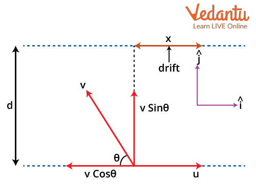
$v_{b / w}$ : Velocity of the boat with respect to the water. This is the velocity the boat's engine provides, i.e., its speed in still water.
$v_{w / g}$ : Velocity of the water with respect to the ground. This is the river's current.
$v_{b / g}$ : Velocity of the boat with respect to the ground. This is the boat's actual, resultant velocity as seen by an observer on the bank.

The relationship connecting them is:
$v_{b / g} = v_{b / w} + v_{w / g}$
This single vector equation governs all boat-river problems.

Boat Crossing a River Problems

The following video from Physics Ninja provides an excellent practical demonstration of the two most common river-crossing scenarios. It visually demonstrates the vector addition and the resulting motion.

Please watch the entire video. It covers two distinct problems: Aiming the boat straight across and drifting downstream. Aiming the boat upstream to travel straight across without any drift.

Now, let's formalize the physics and mathematics behind the two scenarios presented in the video.

Case 1: Crossing in the Shortest Possible Time

Objective: To cross the river of width $d$ in the minimum time.
Analysis: The time to cross depends only on the component of velocity perpendicular to the river banks. Let's set up a coordinate system where the y-axis is straight across the river and the x-axis is along the river bank. The time to cross is $t = d / (v_{b / g})_{y}$ . To minimize $t$ , we must maximize $(v_{b / g})_{y}$ . $(v_{b / g})_{y} = (v_{b / w})_{y} + (v_{w / g})_{y}$ Since the river flows along the x-axis, $(v_{w / g})_{y} = 0$ . Thus, $(v_{b / g})_{y} = (v_{b / w})_{y}$ . The maximum value of $(v_{b / w})_{y}$ is simply the magnitude $v_{b / w}$ , which occurs when the boat is pointed directly across the river (along the y-axis).
Proof & Result:
- Time (Shortest): When $v_{b / w}$ is perpendicular to $v_{w / g}$ , the time to cross is $t_{min} = \frac{d}{v _{b / w}}$ .
- Drift: During this time, the river current carries the boat downstream. The drift $x$ is the displacement along the x-axis: $x = (v_{b / g})_{x} \cdot t_{min}$ . Since $(v_{b / w})_{x} = 0$ in this orientation, $(v_{b / g})_{x} = (v_{w / g})_{x} = v_{w / g}$ .
$x = v_{w / g} \cdot (\frac{d}{v _{b / w}})$

Case 2: Crossing in the Shortest Path (Zero Drift)

Objective: To land at a point directly opposite the starting point.
Analysis: For zero drift, the resultant velocity $v_{b / g}$ must have no component along the river bank. In our coordinate system, this means $(v_{b / g})_{x} = 0$ . $(v_{b / g})_{x} = (v_{b / w})_{x} + (v_{w / g})_{x} = 0$ This implies $(v_{b / w})_{x} = - (v_{w / g})_{x} = - v_{w / g}$ . The boat must have a component of its velocity relative to the water that is directed upstream, exactly canceling the river's flow.
Proof & Result:
- Condition: From the vector diagram, $v_{b / w}$ is the hypotenuse of a right-angled triangle, with $v_{w / g}$ and $v_{b / g}$ as the other two sides. This is only possible if $v_{b / w} > v_{w / g}$ . If the river flows faster than the boat can travel, it's impossible to achieve zero drift.
- Angle: The boat must be aimed upstream at an angle $ϕ$ with respect to the straight-across direction (y-axis), where $sin ϕ = \frac{v _{w / g}}{v _{b / w}}$ .
- Resultant Speed: The speed across the river is $v_{b / g} = v_{b / w}^{2} - v_{w / g}^{2}$ .
- Time: The time taken is $t = \frac{d}{v _{b / g}} = \frac{d}{v _{b / w}^{2} - v _{w g}^{2}}$ . Notice this is longer than the shortest possible time.

Boat-River Problem Vector Diagram — This vector diagram illustrates the setup for a shortest-path (zero drift) crossing. The velocity of the boat relative to water ($\vec{v}_{br}$ in the diagram's notation) must have a component pointing upstream that cancels the river's velocity ($\vec{v}_{r}$), resulting in a net velocity ($\vec{v}_{b}$) that is straight across.

Test your understanding!

A swimmer can swim at a speed of $v$ in still water. They are in a river of width $d$ flowing at speed $u$ . The swimmer wants to cross the river, minimizing their downstream drift. However, $u > v$ . Prove that the minimum possible drift is not zero, and find an expression for this minimum drift.

(Hint: Set up the expression for drift as a function of the angle the swimmer swims relative to the bank, and use calculus to minimize it. This is a challenging problem that requires applying the principles we've discussed.)

Show answer

Let the swimmer swim at an angle $θ$ with respect to the direction straight across the river, pointing upstream. The components of the swimmer's velocity relative to the water are:

Across the river (y-direction): $v_{y} = v cos θ$
Upstream (x-direction): $v_{x} = - v sin θ$

The river flows downstream in the x-direction with speed $u$ . The swimmer's resultant velocity components relative to the ground are:

$(v_{s / g})_{y} = v cos θ$
$(v_{s / g})_{x} = u - v sin θ$

The time to cross the river is determined by the y-component:

t = \frac{d}{( v _{s / g} ) _{y}} = \frac{d}{v cos θ}

During this time, the drift $D$ is the displacement in the x-direction:

D = (v_{s / g})_{x} \cdot t = (u - v sin θ) \frac{d}{v cos θ} = \frac{d}{v} (u sec θ - v tan θ)

To minimize the drift $D$ with respect to the angle $θ$ , we must find where $\frac{d D}{d θ} = 0$ .

\frac{d D}{d θ} = \frac{d}{v} (u sec θ tan θ - v sec^{2} θ) = 0

Since $sec θ \neq = 0$ , we can divide by $sec θ$ :

u tan θ - v sec θ = 0

u \frac{sin θ}{cos θ} - v \frac{1}{cos θ} = 0 ⟹ u sin θ - v = 0

sin θ = \frac{v}{u}

This gives the angle for minimum drift. Note that since $u > v$ , we have $\frac{v}{u} < 1$ , so a real angle $θ$ exists.

Now we find the minimum drift by substituting this back into our expression for $D$ . We need $cos θ$ :

cos θ = 1 - sin^{2} θ = 1 - (\frac{v}{u})^{2} = \frac{u ^{2} - v ^{2}}{u}

So, the minimum drift is:

D_{min} = (u - v \cdot \frac{v}{u}) \frac{d}{v \cdot \frac{u ^{2} - v ^{2}}{u}} = (\frac{u ^{2} - v ^{2}}{u}) \frac{d u}{v u ^{2} - v ^{2}} = \frac{d u ^{2} - v ^{2}}{v}

This confirms that if $u > v$ , the drift can't be zero, and this is its minimum possible value. This problem is similar to 'pr 35' in the Kalda solutions sheet (LINK).

3. The Rain-Person Problem

This is another classic scenario that relies on the direct application of vector subtraction. What an observer experiences as "rain" is the velocity of the rain relative to them.

Let's define the velocities:

$v_{r / g}$ : Velocity of the rain with respect to the ground.
$v_{p / g}$ : Velocity of the person with respect to the ground.
$v_{r / p}$ : Velocity of the rain with respect to the person. This is the apparent velocity of the rain.

The governing equation is:
$v_{r / p} = v_{r / g} - v_{p / g} = v_{r / g} + (- v_{p / g})$
To avoid getting wet, a person must hold their umbrella in the direction opposite to $v_{r / p}$ .

RELATIVE MOTION

The section on 'RAIN PROBLEM' in this document provides a clear derivation and examples for this type of problem.

Please read section '6. RAIN PROBLEM' and its solved examples (21, 22, 23). Pay close attention to the vector diagrams and how an heta is used to find the angle of the apparent rainfall.

The typical problem involves rain falling vertically ( $v_{r / g} = - v_{r} j^$ ) and a person moving horizontally ( $v_{p / g} = v_{p} i^$ ).
The relative velocity is:
$v_{r / p} = (- v_{r} j^) - (v_{p} i^) = - v_{p} i^- v_{r} j^$
The apparent speed of the rain is $∣ v_{r / p} ∣ = v_{p}^{2} + v_{r}^{2}$ .
The rain appears to be coming from an angle $θ$ with the vertical, where:
$tan θ = \frac{∣ ( v _{r / p} ) _{x} ∣}{∣ ( v _{r / p} ) _{y} ∣} = \frac{v _{p}}{v _{r}}$

4. Advanced Application: Pursuit Problems

Let's consider a more advanced problem that is a staple of physics Olympiads. In a pursuit problem, one object's velocity vector always points towards the other object. This means the direction of the relative velocity is continuously changing, often requiring calculus.

Advance Illustrations - Chasing a Cat by a Dog | Kinematics #46 for JEE Advanced

This video from Physics Galaxy tackles a classic pursuit problem: a dog chasing a cat. This is a significant step up in complexity from the constant-velocity problems and demonstrates a powerful problem-solving technique.

Watch the video to see how the problem is set up and solved. The key insight is to switch to the cat's reference frame and analyze the rate at which the separation distance between the dog and cat decreases. This is known as the 'velocity of approach'.

The crucial idea in this problem is to analyze the motion along the line connecting the two objects. Let the separation distance be $L$ . The rate at which this separation decreases is the velocity of approach.
$v_{a pp r o a c h} = - \frac{d L}{d t}$
This velocity of approach is the component of the relative velocity vector along the line joining the objects. In the video's analysis:
$- \frac{d L}{d t} = v_{d o g} - v_{c a t} cos θ$
By integrating this expression (using a clever substitution shown in the video), one can find the total time to catch the cat. This method of analyzing components of relative velocity along and perpendicular to the line of sight is a powerful technique for more complex problems.

Conclusion

In this lesson, we have moved from one-dimensional to two-dimensional relative motion. We've seen that while the core vector equations are simple, their application requires careful geometric and component-wise analysis.

Key Takeaways:

All 2D relative motion problems are governed by the vector equations $v_{A / B} = v_{A} - v_{B}$ and its corollary for nested frames, $v_{A / C} = v_{A / B} + v_{B / C}$ .
For boat-river problems, the resultant velocity is a vector sum of the boat's velocity in water and the water's velocity. We analyzed strategies for achieving the shortest crossing time versus the shortest path (zero drift).
For rain-person problems, the apparent velocity of the rain is a vector subtraction of the person's velocity from the rain's true velocity.
Solving these problems rigorously involves decomposing the vector equations into independent scalar equations for each coordinate axis.

Preview of the Next Lesson:
We've touched upon the concept of "velocity of approach." In our next lesson, we will formalize this and use it to solve another classic type of 2D problem: deriving and applying the condition for the minimum separation distance between two objects in uniform 2D motion. We will see that the minimum distance occurs precisely when the velocity of approach becomes zero.

Recommended resources