Angular Kinematics: Definitions and Calculus Relationships

1. Describing Position on a Circle: Angular Position and Polar Coordinates

When a particle moves in a 2D plane, we typically use Cartesian coordinates $(x,y)$. However, for motion constrained to a circular path, this system is cumbersome. A more natural choice is the polar coordinate system $(r,\theta )$.

• $r$: The radial distance from the origin.
• $\theta$: The angle measured counter-clockwise from a reference axis (usually the positive x-axis).

For a particle moving in a circle of radius $R$ centered at the origin, the radial coordinate is constant: $r=R$. The particle's location is therefore completely specified by a single variable: the angle $\theta$. We call this the angular position. By convention, $\theta$ is positive for counter-clockwise (CCW) rotation and negative for clockwise (CW) rotation. The natural unit for angular position in physics is the radian, as it simplifies calculus operations.

To perform calculus, we need to express vectors. In Cartesian coordinates, the unit vectors $\hat{i}$ and $\hat{j}$ are constant. A key difference in polar coordinates is that the unit vectors, ${\hat{u}}_r$ (radial) and ${\hat{u}}_{\theta }$ (tangential), change direction as the particle moves.

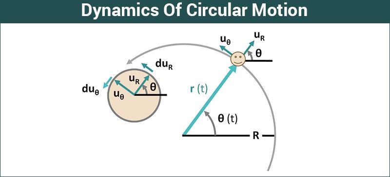
The following reading establishes the mathematical definitions for polar coordinates and their unit vectors. Your background in trigonometry will make this straightforward.

From the reading, the key relationships are:

• ${\hat{u}}_r=(\cos \theta )\hat{i}+(\sin \theta )\hat{j}$
• ${\hat{u}}_{\theta }=-(\sin \theta )\hat{i}+(\cos \theta )\hat{j}$

Crucially, because $\theta$ is a function of time, $\theta (t)$, these unit vectors are also functions of time. This means their time derivatives are non-zero, a fact we will now use to derive velocity.

2. Angular Velocity: The Rate of Change of Angular Position

Just as linear velocity is the time derivative of position, angular velocity is the time derivative of angular position. We denote it by the Greek letter omega, $\omega$.

For the rigorous derivation you prefer, let's start from the fundamental definition of the velocity vector, $\vec{v}=\frac{d\vec{r}}{dt}$.

The position vector $\vec{r}$ in polar coordinates is elegantly simple:
$\vec{r}(t)=r{\hat{u}}_r(t)$
For circular motion of radius $R$, this becomes $\vec{r}(t)=R{\hat{u}}_r(t)$.

To find the velocity, we differentiate this with respect to time. Since $R$ is constant, we use the chain rule on ${\hat{u}}_r(t)$. The following video provides a step-by-step derivation.

As demonstrated in the video, the derivation proceeds as follows:

1. Start with the position vector: $\vec{r}(t)=R{\hat{u}}_r(t)=R(\cos \theta (t)\hat{i}+\sin \theta (t)\hat{j})$.
2. Differentiate with respect to time, applying the chain rule:
   $\vec{v}(t)=\frac{d\vec{r}}{dt}=R\left(-\sin \theta (t)\frac{d\theta }{dt}\hat{i}+\cos \theta (t)\frac{d\theta }{dt}\hat{j}\right)$
3. Factor out the common term $\frac{d\theta }{dt}$:
   $\vec{v}(t)=R\frac{d\theta }{dt}\left(-\sin \theta (t)\hat{i}+\cos \theta (t)\hat{j}\right)$
4. Recognize that the term in the parenthesis is the definition of the tangential unit vector, ${\hat{u}}_{\theta }$.

This gives us the final expression for the velocity vector and formally defines angular velocity, $\omega$:

$\omega \equiv \frac{d\theta }{dt}$
$\vec{v}(t)=R\omega (t){\hat{u}}_{\theta }(t)$

This elegant result proves that for circular motion, the velocity vector is always tangential to the circle, with a magnitude $v=|R\omega |$.

The Vector Nature of Angular Velocity

So far, we've treated $\omega$ as a scalar. However, it is the component of a vector, $\vec{\omega }$. For motion in the $xy$-plane, the angular velocity vector $\vec{\omega }$ points along the axis of rotation (the z-axis). Its direction is given by the right-hand rule: if you curl the fingers of your right hand in the direction of rotation, your thumb points in the direction of $\vec{\omega }$.

• Counter-clockwise rotation: $\omega >0$, $\vec{\omega }$ points in the $+\hat{k}$ direction.
• Clockwise rotation: $\omega <0$, $\vec{\omega }$ points in the $-\hat{k}$ direction.

This vector definition is essential for more advanced 3D rotational dynamics.

3. Angular Acceleration: The Rate of Change of Angular Velocity

The analogy to linear motion continues. Angular acceleration, denoted by the Greek letter alpha ($\alpha$), is the time derivative of angular velocity.

$\alpha \equiv \frac{d\omega }{dt}=\frac{d}{dt}\left(\frac{d\theta }{dt}\right)=\frac{d^2\theta }{d{t}^2}$

This completes the trio of angular kinematic quantities and their calculus-based relationships:

• Angular Position: $\theta (t)$
• Angular Velocity: $\omega (t)=\frac{d\theta }{dt}$
• Angular Acceleration: $\alpha (t)=\frac{d\omega }{dt}=\frac{d^2\theta }{d{t}^2}$

Like angular velocity, angular acceleration is also a vector, $\vec{\alpha }$, pointing along the axis of rotation ($\vec{\alpha }=\alpha \hat{k}$ for planar motion). The sign of $\alpha$ tells us how the angular velocity is changing.

• If $\vec{\omega }$ and $\vec{\alpha }$ have the same direction (e.g., both $+\hat{k}$), the object's rotation is speeding up.
• If $\vec{\omega }$ and $\vec{\alpha }$ have opposite directions, the object's rotation is slowing down.

The same MIT notes explain this concept.

4. From Acceleration to Position: The Integral Relationships

The calculus relationships work in reverse, too. Just as we did for linear motion, we can find changes in angular velocity and position by integrating over time.

Given angular acceleration $\alpha (t)$, the change in angular velocity from time $t=0$ to time $t$ is:
$\Delta \omega =\omega (t)-{\omega }_0={\int }_0^t\alpha (t^{\prime })d{t}^{\prime }$

Similarly, given angular velocity $\omega (t)$, the angular displacement is:
$\Delta \theta =\theta (t)-{\theta }_0={\int }_0^t\omega (t^{\prime })d{t}^{\prime }$

These integral forms are essential for solving problems where acceleration or velocity are functions of time.

This confirms that the entire calculus framework you mastered for 1D kinematics has a direct and powerful analogue in rotational kinematics.

Conclusion

In this lesson, we have laid the mathematical groundwork for describing circular motion. By adopting polar coordinates and rigorously applying calculus, we have seen how the concepts of position, velocity, and acceleration are transformed for rotation.

Key Takeaways:

• Circular motion is described by angular position $\theta$, angular velocity $\omega$, and angular acceleration $\alpha$.
• These quantities are connected by the same calculus relationships as their linear counterparts: $\omega =\frac{d\theta }{dt}$ and $\alpha =\frac{d\omega }{dt}=\frac{d^2\theta }{d{t}^2}$.
• The derivation of the linear velocity vector $\vec{v}$ for circular motion requires differentiating the time-varying polar unit vectors, which rigorously proves that $\vec{v}=R\omega {\hat{u}}_{\theta }$.
• Angular velocity $\vec{\omega }$ and angular acceleration $\vec{\alpha }$ are vectors directed along the axis of rotation, with their direction determined by the right-hand rule.

Preview of the Next Lesson:
We have derived the velocity vector $\vec{v}$ for a particle in circular motion. The logical next step is to find its acceleration vector, $\vec{a}=\frac{d\vec{v}}{dt}$. This will be more involved than finding $\vec{v}$, because now we must differentiate a product of two time-dependent functions, $\omega (t)$ and ${\hat{u}}_{\theta }(t)$. This differentiation will reveal two distinct components of acceleration. In our next lesson, we will prove the formula for centripetal acceleration ($a_c=v^2/r$) using vector methods, which will emerge directly from this derivation.