Verifying Kinematics Solutions

1. Dimensional Analysis: The Grammar of Physics

The fundamental principle behind dimensional analysis is dimensional homogeneity: any physically meaningful equation must have the same dimensions on both sides. You cannot add a length to a time, nor can you equate mass with velocity. This simple rule is surprisingly powerful.

In mechanics, most quantities can be expressed in terms of three fundamental dimensions:

• Mass ($M$)
• Length ($L$)
• Time ($T$)

For example, the dimensions of velocity are $[v]=L/T$, and the dimensions of force are $[F]=[ma]=M\cdot L/T^2$.

1.1 Application 1: Checking the Consistency of Equations

The most direct use of dimensional analysis is to verify that your final answer or an intermediate equation is dimensionally correct. If it isn't, you've made a mistake.

Let's watch a short video that demonstrates this by checking a familiar kinematic equation.

As you saw, by reducing each term to its fundamental dimensions ($L,T$), you can ensure the equation is consistent. Let's try it with another equation we derived: v_f^2 - v_i^2 = 2a\Delta x.

• Left side: $[v^2]=(L/T{)}^2=L^2/T^2$.
• Right side: $[a\Delta x]=(L/T^2)\cdot L=L^2/T^2$.
  The dimensions match, which gives us confidence in the formula's structure.

1.2 Application 2: Deriving Functional Relationships

A more sophisticated use of dimensional analysis allows you to determine the form of an equation, up to a dimensionless constant. This is a powerful way to understand how a physical quantity depends on other parameters, even before solving the problem rigorously.

The foundational text for this section is David Morin's Introduction to Classical Mechanics. His chapter on problem-solving strategies is exceptionally clear and aligns perfectly with the rigorous approach you prefer.

To summarize Morin's method:

1. Identify all the physical parameters the result could depend on.
2. Assume a product of powers for the relationship, e.g., $f\propto R^a{\rho }^b{G}^c$.
3. Equate the dimensions on both sides of the equation.
4. Solve the resulting system of linear equations for the exponents $a,b,c$.

Test your understanding!

Let's apply this method to the problem shown in the image below. A naive model for the radius $R$ of a blast wave from an explosion suggests it depends only on the energy released $E$, the density of the medium $\rho$, and the time elapsed $t$. The relationship is $R=C\cdot E^a{\rho }^b{t}^c$, where $C$ is a dimensionless constant.

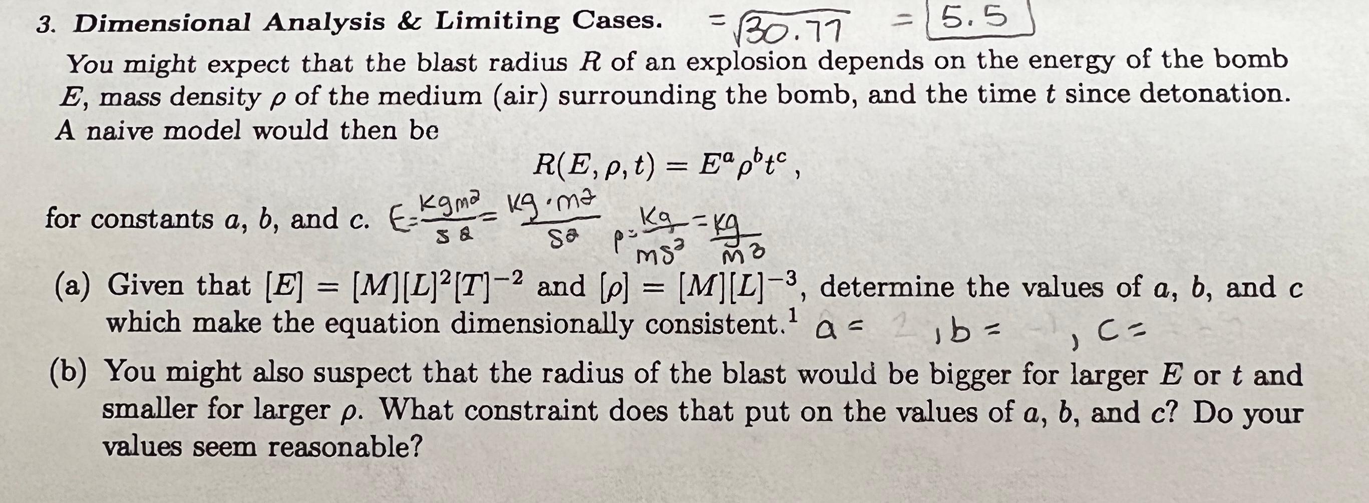
Using the dimensions $[E]=M{L}^2{T}^{-2}$ and $[\rho ]=M{L}^{-3}$, determine the exponents $a$, $b$, and $c$.

Show answer

We start by setting up the dimensional equation:
$[R]=[E{]}^a[\rho {]}^b[t{]}^c$
$L^1{M}^0{T}^0=(M{L}^2{T}^{-2}{)}^a(M{L}^{-3}{)}^b(T{)}^c$
$L^1{M}^0{T}^0=M^{a+b}{L}^{2a-3b}{T}^{-2a+c}$

Now, we equate the exponents for each fundamental dimension:

1. Mass (M): $0=a+b$
2. Length (L): $1=2a-3b$
3. Time (T): $0=-2a+c$

From equation (1), we get $b=-a$.
Substitute this into equation (2): $1=2a-3(-a)=2a+3a=5a$.
This gives us $a=1/5$.
Therefore, $b=-1/5$.
From equation (3), $c=2a=2(1/5)$. This gives us $c=2/5$.

So, the relationship is $R\propto E^{1/5}{\rho }^{-1/5}{t}^{2/5}$, or $R\propto {\left(\frac{E{t}^2}{\rho }\right)}^{1/5}$.
This famous result was used by G.I. Taylor to estimate the yield of the first atomic bomb using only declassified photographs.

1.3 A Deeper Look: The Buckingham Pi Theorem

For a mathematically complete perspective, we can introduce the Buckingham $\Pi$ Theorem. It provides a formal method for determining how many independent dimensionless groups can be formed from a set of variables.

Theorem: If a physical system involves $N$ variables and $D$ independent fundamental dimensions (like M, L, T), then you can form $k=N-D$ independent dimensionless quantities (often denoted ${\Pi }_1,{\Pi }_2,...,{\Pi }_k$). The general relationship between the variables can then be expressed as a function of these dimensionless groups, e.g., $f({\Pi }_1,{\Pi }_2,...,{\Pi }_k)=0$.

In the blast wave example, we had $N=4$ variables ($R,E,\rho ,t$) and $D=3$ dimensions ($M,L,T$). Thus, we can form $k=4-3=1$ dimensionless group. This group is ${\Pi }_1=R\cdot E^{-1/5}{\rho }^{1/5}{t}^{-2/5}$. Since there's only one such group, it must be equal to a constant, which immediately gives us the relationship we found.

2. Limiting Case Analysis: The Sanity Check

While dimensional analysis validates the structure of a formula, limiting case analysis validates its physical behavior. The idea is to test your formula in extreme scenarios where you already know what the answer should be. If your formula doesn't simplify to the known result, it's wrong.

Let's explore this powerful technique with another excerpt from Morin's book.

The key takeaways from the reading are:

• Check known points: If a parameter goes to zero or infinity, does your formula reduce to a simpler, known equation?
• Use Taylor series: For limits where a dimensionless parameter $ϵ\ll 1$, approximations like $(1+ϵ{)}^n\approx 1+nϵ$, $\sin (ϵ)\approx ϵ$, and $e^{ϵ}\approx 1+ϵ$ are essential tools.
• Build intuition: This process forces you to think about the physical meaning of your result.

3. Synthesis: A JEE-Style Application

In multiple-choice questions, you can often find the correct answer purely by elimination, using a combination of dimensional and limiting case analysis, without solving the problem from scratch.

Problem:
A person throws a ball with speed $v$ from the edge of a cliff of height $h$. To achieve the maximum horizontal distance, they throw it at a certain optimal angle. Which of the following expressions could represent this maximum horizontal distance, $R_{max}$?

(a) $\frac{g{h}^2}{v^2}$
(b) $\frac{v^2}{g}$
(c) $\frac{v^2}{g}\sqrt{1+\frac{2gh}{v^2}}$
(d) $\frac{v^2}{g}\left(1+\frac{2gh}{v^2}\right)$

Let's analyze the options systematically:

1. Dimensional Analysis: The target quantity, range, has dimensions of length $[L]$.

   • (a) $[g{h}^2/v^2]=(L/T^2)\cdot L^2/(L/T{)}^2=L$. Dimensionally possible.
   • (b) $[v^2/g]=(L/T{)}^2/(L/T^2)=L$. Dimensionally possible.
   • (c) $\frac{2gh}{v^2}$ is dimensionless, so the term under the square root is dimensionless. The expression has dimensions of $[v^2/g]=L$. Dimensionally possible.
   • (d) Same as (c). Dimensionally possible.
     Dimensional analysis alone is not enough here.

2. Limiting Case Analysis:

   • Case 1: No cliff ($h\to 0$)
     The problem becomes finding the maximum range on level ground. You may recall from projectile motion that this is $R_{max}=v^2/g$ (achieved at a 45° angle). Let's see which formulas reduce to this.

     • (a) $R_{max}\to 0$. Incorrect.
     • (b) $R_{max}=v^2/g$. This matches. A possible candidate.
     • (c) $R_{max}\to \frac{v^2}{g}\sqrt{1+0}=\frac{v^2}{g}$. This also matches. A possible candidate.
     • (d) $R_{max}\to \frac{v^2}{g}(1+0)=\frac{v^2}{g}$. This also matches. A possible candidate.
       We have eliminated (a).

   • Case 2: Zero initial speed ($v\to 0$)
     If you drop the ball from the cliff edge with no speed, it should land directly at the base. The horizontal range must be 0.

     • (b) $R_{max}\to 0$. This works.
     • (c) $R_{max}=\frac{v}{g}\sqrt{v^2+2gh}$. As $v\to 0$, this becomes $0\cdot \sqrt{2gh}=0$. This works.
     • (d) $R_{max}=\frac{v^2}{g}+2h$. As $v\to 0$, this becomes $2h$. This is incorrect. The range should be 0.
       We have eliminated (d). We are left with (b) and (c).

   • Final Check: Option (b), $R_{max}=v^2/g$, does not depend on the height $h$. This is physically unreasonable. A greater cliff height should allow for a greater maximum range. Option (c) is the only one remaining that correctly handles both limiting cases and depends on $h$. Therefore, (c) must be the correct answer.

Conclusion

Today, we've explored two powerful techniques for validating your work and deepening your physical understanding. These are not just tricks; they are fundamental aspects of thinking like a physicist.

Key Takeaways:

• Dimensional Analysis ensures your equations are structurally sound. It allows you to check for consistency and even derive the functional form of an answer by equating the powers of $M$, $L$, and $T$.
• Limiting Case Analysis ensures your equations behave correctly in simple or extreme scenarios. It provides a robust "sanity check" by comparing your result to known physics.
• Combined Use: Together, these methods form a powerful strategy for verifying solutions and even deducing answers in multiple-choice settings, a critical skill for competitive exams.

As Kevin Zhou notes in his Olympiad handouts, dimensional analysis and limiting cases are not just techniques but "ways of life". I encourage you to apply them to every problem you solve from now on.

Preview of the Next Lesson:

We have now concluded our deep dive into the calculus and analytical methods of one-dimensional kinematics. We will now move on to Module 3: Graphical Analysis in Kinematics. In the next lesson, we will rigorously prove the integral and derivative relationships between position-time ($x-t$), velocity-time ($v-t$), and acceleration-time ($a-t$) graphs. This will provide a visual and often more intuitive pathway to solving the same kinds of complex problems we've been analyzing with calculus.