Calculus of Kinematics Graphs

1. The Derivative Relationship: Slope as Instantaneous Rate of Change

Let's begin by proving the connection between the slope of a kinematic graph and the instantaneous rate of change.

1.1 From Position to Velocity

Recall the definition of average velocity, $\bar{v}$, over a time interval $\Delta t=t_2-t_1$:
$\bar{v}=\frac{\Delta x}{\Delta t}=\frac{x(t_2)-x(t_1)}{t_2-t_1}$
Geometrically, on a position-time (x-t) graph, this is the slope of the secant line connecting the points $(t_1,x(t_1))$ and $(t_2,x(t_2))$.

To find the instantaneous velocity at a single moment in time, say $t_1$, we must shrink the interval $\Delta t$ to be infinitesimally small. As we let $\Delta t\to 0$, the secant line pivots and approaches the tangent line to the curve at the point $(t_1,x(t_1))$.

In the language of calculus, this is the definition of the derivative:
$v(t)={\lim }_{\Delta t\to 0}\frac{\Delta x}{\Delta t}=\frac{dx}{dt}$

Since the derivative $\frac{dx}{dt}$ gives the instantaneous velocity and also represents the slope of the tangent line to the x-t graph, we have our first proof.

Proof 1: The instantaneous velocity $v(t)$ is equal to the slope of the tangent line to the position-time graph at time $t$.

1.2 From Velocity to Acceleration

The exact same logic applies to the relationship between velocity and acceleration. Instantaneous acceleration is the rate of change of velocity:
$a(t)={\lim }_{\Delta t\to 0}\frac{\Delta v}{\Delta t}=\frac{dv}{dt}$

Proof 2: The instantaneous acceleration $a(t)$ is equal to the slope of the tangent line to the velocity-time graph at time $t$.

To see a detailed, formal derivation of these concepts starting from first principles, please read the following text. It rigorously develops the idea of instantaneous velocity from average velocity using limit arguments, which is the core of our proof.

The key takeaway is that the "slope" of a curve at a point is a geometric interpretation of the derivative. Thus, the derivative relationships $v=dx/dt$ and $a=dv/dt$ directly imply that the slope of an x-t graph gives velocity, and the slope of a v-t graph gives acceleration.

2. The Integral Relationship: Area as Net Change

Now, let's prove the inverse relationship: the connection between the area under a curve and the net change in a kinematic quantity. This proof relies on the Fundamental Theorem of Calculus.

2.1 From Acceleration to Velocity

We start with the definition of acceleration:
$a(t)=\frac{dv}{dt}$
We can rewrite this in differential form as $dv=a(t)dt$. To find the total change in velocity, $\Delta v$, between two times $t_1$ and $t_2$, we integrate both sides:
${\int }_{v_1}^{v_2}dv={\int }_{t_1}^{t_2}a(t)dt$
$v_2-v_1={\int }_{t_1}^{t_2}a(t)dt$
$\Delta v={\int }_{t_1}^{t_2}a(t)dt$
The definite integral on the right-hand side is, by definition, the signed area under the a-t curve between $t_1$ and $t_2$.

Proof 3: The net change in velocity $\Delta v$ over a time interval is equal to the signed area under the acceleration-time graph over that interval.

2.2 From Velocity to Displacement

The same proof structure holds for the relationship between velocity and position. We start with $v(t)=\frac{dx}{dt}$, rewrite it as $dx=v(t)dt$, and integrate:
${\int }_{x_1}^{x_2}dx={\int }_{t_1}^{t_2}v(t)dt$
$x_2-x_1={\int }_{t_1}^{t_2}v(t)dt$
$\Delta x={\int }_{t_1}^{t_2}v(t)dt$
The term $\Delta x=x_2-x_1$ is the displacement.

Proof 4: The displacement $\Delta x$ over a time interval is equal to the signed area under the velocity-time graph over that interval.

To understand how this integration works visually, consider approximating the area under a curve with a series of thin rectangles, a method known as a Riemann sum.

For a rigorous and concise proof using the Fundamental Theorem of Calculus, please study the following material.

It is crucial to distinguish between displacement and distance. Displacement ($\Delta x$) is the net change in position, a vector quantity. The area under the v-t graph gives you displacement, meaning area below the t-axis is counted as negative. Distance is the total path length, a scalar. To find the total distance from a v-t graph, you must take the absolute value of the velocity, which means treating all areas as positive:
$\text{Distance}={\int }_{t_1}^{t_2}|v(t)|dt$

3. Synthesis: The Complete Picture

The derivative and integral relationships are two sides of the same coin, elegantly captured by the Fundamental Theorem of Calculus. One operation "undoes" the other.

• Differentiation: x-t $\stackrel{\text{slope}}{\to }$ v-t $\stackrel{\text{slope}}{\to }$ a-t
• Integration: a-t $\stackrel{\text{area}}{\to }$ $\Delta v$ (on v-t graph) $\stackrel{\text{area}}{\to }$ $\Delta x$ (on x-t graph)

The following image provides an excellent summary of these interconnected relationships for a sample motion.

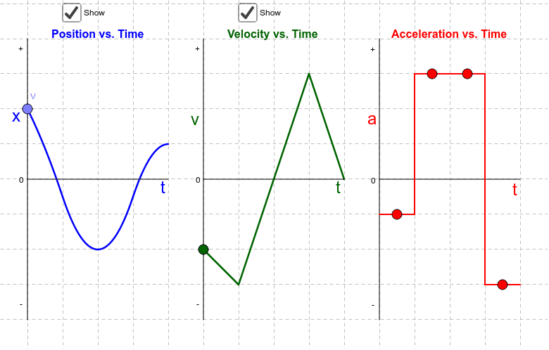
Let's trace a few points on these graphs to solidify the concepts:

• In the first segment (0-2s), the acceleration is a positive constant. This means the slope of the v-t graph is a positive constant (a straight line) and the v-t graph value increases linearly. The x-t graph, whose slope must be increasing, is therefore an upward-curving parabola.
• At t=4s, the v-t graph is at its peak and has a slope of zero. Correspondingly, the a-t graph has a value of zero at t=4s. The x-t graph has its steepest positive slope at this point, indicating maximum positive velocity.
• Between t=6s and t=8s, the velocity is a negative constant. The slope of the x-t graph is therefore a negative constant (a straight line sloping down). The slope of the v-t graph is zero, so the acceleration is zero. The area under the v-t graph here is $(-2\text{ m/s})\times (2\text{ s})=-4\text{ m}$. This is the displacement during this interval.

Conclusion

In this lesson, we have rigorously established the fundamental links between the graphical representations of motion and the calculus that underpins them. These are not merely convenient rules but direct consequences of the mathematical definitions of the derivative and the integral.

Key Takeaways:

• Derivative as Slope: The instantaneous velocity $v(t)$ is the slope of the position-time graph. The instantaneous acceleration $a(t)$ is the slope of the velocity-time graph. This is a geometric consequence of the definition $v=dx/dt$ and $a=dv/dt$.
• Integral as Area: The change in velocity $\Delta v$ is the area under the acceleration-time graph. The displacement $\Delta x$ is the area under the velocity-time graph. This is proven by the Fundamental Theorem of Calculus, which connects the integral ($\int f(t)dt$) to the antiderivative.
• Inverse Relationship: Differentiation and integration are inverse operations. Finding the slope of a graph moves you "down" the kinematic chain (from x to v to a), while finding the area moves you "up" (from a to v to x).

Preview of the Next Lesson:

Having proven why these relationships hold, we will now put them into practice. In the next lesson, we will focus on applying these rules to construct accurate kinematic graphs (x-t, v-t, a-t) from complex verbal or mathematical descriptions of motion. This will be a critical skill for visualizing and solving advanced problems.