Hello! Welcome to our third lesson in the "Graphical Analysis in Kinematics" module.
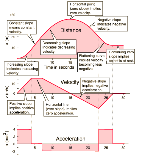
In our previous session, we established a systematic method for constructing a full set of kinematic graphs (, , ) from either a verbal or mathematical description of motion. We focused on translating the physics into the correct graphical shapes, leveraging the derivative and integral relationships we had proved.
Today, we will invert the process. Instead of creating the graphs, we will start with them and learn how to extract precise quantitative information, such as displacement, distance, change in velocity, and instantaneous acceleration. This skill is about reading the "story" of motion told by the graphs and calculating key numerical values directly from their geometric properties. Mastering this is crucial for solving many JEE Advanced problems with efficiency and deep physical insight.
1. The Two Pillars of Graphical Analysis: Slope and Area
As we've established, the entire framework of kinematic graphical analysis rests on the fundamental calculus relationships between position, velocity, and acceleration. Let's formalize the two main operations we can perform on these graphs to extract numbers.
A. Slope: Measuring Instantaneous Rates of Change
The derivative of a function at a point gives the slope of the tangent line at that point. This provides a powerful geometric tool:
- Velocity from Position-Time (x-t) Graph: The instantaneous velocity at any time is the slope of the tangent to the graph at that time.
- Acceleration from Velocity-Time (v-t) Graph: Similarly, the instantaneous acceleration at any time is the slope of the tangent to the graph at that time.
The following video provides a clear walkthrough of these concepts.
Kinematics Graphs in 1 Shot 🔥 | One Shot JEE Advanced 2020 Revision | IIT JEE Physics | Vedantu
Let's watch a segment from the 'Kinematics Graphs in 1 Shot' video by Vedantu Momentum. It clearly demonstrates how to find average and instantaneous velocity from the slope of an x-t graph.
Watch from 03:08 to 06:23 to see how the slope of a chord (secant line) gives average velocity, and from 12:00 to 14:26 to see how the slope of the tangent gives instantaneous velocity. Pay close attention to the convention of measuring the angle with the positive time-axis.
Inferring Acceleration from the x-t Graph
Since , the acceleration is related to the rate of change of the slope of the graph, which is its curvature.
- If the graph is concave up (curving upwards, like a smiling mouth), its slope is increasing. This means velocity is increasing, so the acceleration is positive.
- If the graph is concave down (curving downwards, like a frowning mouth), its slope is decreasing. This means velocity is decreasing, so the acceleration is negative.
- An inflection point (where curvature changes) on the graph corresponds to a point of zero acceleration.
For a rigorous explanation of this relationship, please read the following text.
The LibreTexts page 'Acceleration' provides a formal connection between the curvature of a position-time graph and the sign of acceleration.
Read the first two paragraphs of the section, starting from 'You can probably figure out on your own now...' up to '...motion with constant velocity'. This text formally describes how concavity relates to the sign of acceleration.
B. Area: Measuring Net Change
The Fundamental Theorem of Calculus tells us that the definite integral of a rate function gives the net change in the original quantity. Geometrically, this is the area under the curve.
- Displacement from Velocity-Time (v-t) Graph: The displacement over a time interval is the signed area under the graph during that interval.
- Change in Velocity from Acceleration-Time (a-t) Graph: The change in velocity is the signed area under the graph.
Displacement vs. Distance
This is a critical distinction for quantitative problems.
- Displacement () is the net change in position. It is calculated as the signed area: area above the time axis is positive, and area below is negative.
- Distance is the total path length traveled. It is calculated as the sum of the magnitudes of the areas: all areas are treated as positive.
The following video segments explain these area relationships and the crucial difference between displacement and distance.
Kinematics Graphs in 1 Shot 🔥 | One Shot JEE Advanced 2020 Revision | IIT JEE Physics | Vedantu
Let's return to the Vedantu video to see the area concepts in action.
Watch the following segments: 18:13 to 23:27: This part explains that area under the v-t graph is displacement, with a brief mention of the integral relationship. 23:27 to 26:38: This is a crucial section. Pay close attention to how displacement (signed area) and total distance traveled (sum of absolute areas) are calculated differently when the velocity changes sign. 26:38 to 31:46: This section demonstrates that the area under the a-t graph gives the change in velocity (v_f - v_i), not the velocity itself. This is a common trap in problems.
2. Analysis of Non-Standard Graphs
JEE Advanced problems often go beyond graphs of , , and versus time. You may encounter graphs like vs. , vs. , or vs. . Analyzing these requires applying the chain rule, a tool you're very familiar with from mathematics.
The key relationship we need is for acceleration:
Using the chain rule, we can express this in terms of position :
Since , we arrive at the master equation for non-standard graphs:
Let's see how this is used.
A. Velocity vs. Position (v-x) Graph
On a graph, the slope of the tangent is . To find the acceleration at a point :
- Read the velocity from the vertical axis (the y-coordinate of the point).
- Calculate the slope of the tangent, , at that point.
- The acceleration is the product of these two values: .
B. vs. Position () Graph
This graph has a remarkably direct relationship with acceleration. Let's find the slope of this graph, .
Using the chain rule again:
Recognizing that , we get:
Thus, the acceleration is simply half the slope of the graph.
C. Acceleration vs. Position (a-x) Graph
Here, we're interested in the area under the curve. We start with our master equation and rearrange it for integration:
Now, we integrate both sides between an initial state and a final state :
Evaluating the integrals gives:
The area under the a-x graph gives the change in , which you might recognize as the change in kinetic energy per unit mass.
The next video clip provides derivations and worked examples for all three of these non-standard graph types.
Kinematics Graphs in 1 Shot 🔥 | One Shot JEE Advanced 2020 Revision | IIT JEE Physics | Vedantu
The final segments of the Vedantu video are dedicated to these advanced graph types common in JEE.
Watch carefully from 32:18 to 43:21. The presenter will cover: v-x graphs (32:18 - 36:28) v²-x graphs (36:28 - 41:25) a-x graphs (41:25 - 43:21) Follow the derivations closely, as they are direct applications of calculus.
Test your understanding!
The graphs for two objects, A and B, are shown. Both objects start from the same position at .
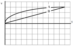
- Which object has a greater acceleration at the moment they have the same velocity?
- Which object has traveled a greater distance at the moment they have the same velocity?
Show answer
-
Acceleration: Acceleration is the slope of the graph.
- Object A's graph is a straight line with a constant positive slope. So, .
- Object B's graph is a horizontal line, so its slope is zero. Thus, .
- Therefore, at the moment of intersection (when velocities are equal), object A has a greater acceleration.
-
Distance: Distance traveled is the area under the graph.
- At the time of intersection, let's call it , the area under graph B is a rectangle with area .
- The area under graph A is a triangle with area .
- Since , object B has traveled a greater distance when their velocities become equal.
3. Synthesis: A JEE-Level Problem
Let's apply these principles to a problem that requires you to correlate different types of graphs for the same motion, a classic JEE question style.
Test your understanding! (JEE Main 2018)
The image below shows four graphs representing the same one-dimensional motion. Which of the graphs is incorrect?

Hint: Start by analyzing the simplest graph, the v-t graph (d), to understand the story of the motion. Then, check if the other graphs tell the same story using the rules of slope and area.
Show answer
Let's analyze the motion from graph (d), the v-t graph:
- From to : The velocity is positive but decreases linearly from to 0. This means the object is moving in the positive direction while slowing down with constant negative acceleration.
- At : The velocity is momentarily zero. The object is at rest.
- From to : The velocity is negative and its magnitude increases linearly from 0 to . This means the object is now moving in the negative direction, speeding up with the same constant negative acceleration.
Now let's check the other graphs for consistency.
-
Graph (c), x-t:
- This is a downward-opening parabola, which correctly represents motion with constant negative acceleration ().
- The slope at is positive ().
- The slope at is zero, corresponding to the peak of the parabola, where .
- The slope for is negative and increasing in magnitude. This graph is consistent.
-
Graph (a), v-x:
- This is a vs. graph. We can use the relation . Since is constant and negative, we have . Integrating gives , or .
- This is the equation of a parabola with its axis along the x-axis. The graph shown is indeed a parabola on its side. As increases from 0, decreases from to 0. Then as decreases back towards 0, becomes negative. This graph is consistent.
-
Graph (b), distance-t:
- Distance is the total path length and can never decrease.
- From to , the object moves away from the origin, so distance = position. The graph should be a parabola curving downwards.
- From to , the object moves back towards the origin. The total distance traveled continues to increase. The slope of the distance-t graph is speed, .
- According to graph (d), the speed at is . However, graph (b) shows a slope of zero at . The tangent at the origin is horizontal.
- This is a contradiction. The initial slope of the distance-time graph should be . Therefore, graph (b) is incorrect.
Conclusion
In this lesson, we have armed ourselves with the tools to perform quantitative analysis on any kinematic graph you might encounter. By understanding the physical meaning of slope and area, we can bypass complex algebraic calculations and solve problems more directly and intuitively.
Key Takeaways:
- Slope is Rate: The slope of a tangent on a kinematic graph always represents the instantaneous rate of change (e.g., ).
- Area is Change: The area under a graph between two points represents the net change in the integrated quantity (e.g., ).
- Displacement vs. Distance: Displacement is the signed area under the graph, while distance is the sum of the absolute areas.
- Non-Standard Graphs: For graphs not plotted against time, use the relation and its integrated forms to find quantitative information. The relationships for and graphs are particularly powerful shortcuts.
Preview of the Next Lesson:
We have now learned how to construct graphs and how to extract data from them. In our next lesson, we will combine these skills to solve problems involving piecewise motion by analyzing and connecting corresponding graph segments. We will tackle complex scenarios where the motion changes character (e.g., acceleration changes abruptly), a common feature in advanced problems.