Analyzing Piecewise Motion Graphs

Hello! Welcome to the fourth lesson in our module on Graphical Analysis in Kinematics.

In our last session, you mastered the art of extracting quantitative data from kinematic graphs by analyzing their slopes and areas. We saw how this graphical calculus provides a powerful alternative to purely algebraic methods.

Today, we will synthesize these skills to tackle piecewise motion. These are scenarios where an object's motion changes its character—for instance, a car accelerating, then cruising, then braking. Each "piece" of the motion follows a different rule. Your goal is to solve problems involving such motion by analyzing the individual graph segments and, crucially, understanding how they connect.

Given your strength in mathematics, you will recognize this as the physical application of piecewise functions. We will rigorously examine the points where the graph segments join, using the concepts of continuity and differentiability to understand what is physically happening at the moments of transition.

1. The Mathematics of Connecting Segments

When the rule of motion changes, what happens at the boundary? For example, if a rocket's engine cuts out, the acceleration changes abruptly. How is this reflected in the graphs? The answer lies in the mathematical properties of continuity and differentiability.

To build a rigorous foundation, let's explore these concepts formally.

Continuity and differentiability of a function

The document 'Continuity and differentiability of a function' provides the precise mathematical definitions we need. It also includes a section on kinematic interpretation, making it directly relevant.

Please study the following sections from this PDF: Section 1.2, 'Continuity at a point': Focus on the definition lim x→a f(x) = f(a) and the graphical idea of an 'unbroken curve'. Note the example of a 'jump' discontinuity. Section 1.5, 'Continuity and differentiability': Absorb the key theorem: Differentiability implies continuity, but the converse is false. Pay close attention to the example of a 'corner' or 'cusp' where a function is continuous but not differentiable. Section 2.1, 'Definition' (of Differentiability): Review the limit definition of the derivative. Note the example of a piecewise function and the method used to check for differentiability at the connecting point by comparing left-hand and right-hand derivatives. Section 2.2.3, 'Kinematic interpretation': This small but vital section explicitly links the derivative to velocity and acceleration.

Now, let's apply these mathematical principles to our kinematic graphs:

Position-Time (x-t) Graph:
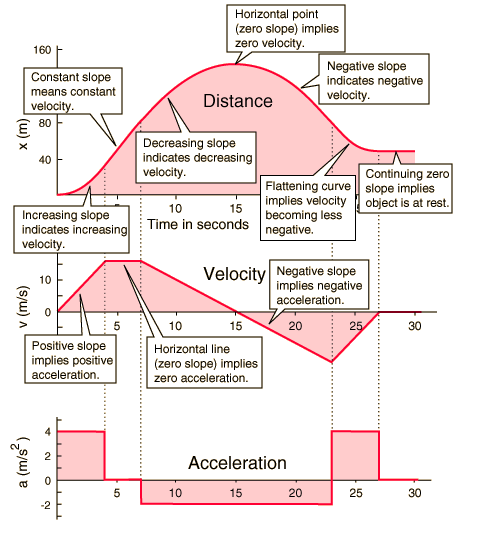
- Continuity: The position of a physical object must be a continuous function of time. An object cannot teleport. A jump discontinuity in an $x - t$ graph is physically impossible.
- Differentiability: The $x - t$ graph is not always differentiable. A "corner" on the $x - t$ graph implies that the slope changes abruptly. Since slope = velocity, this represents an instantaneous change in velocity. This is a common physical approximation, such as a perfectly elastic bounce off a wall.
Velocity-Time (v-t) Graph:
- Continuity: Velocity can be discontinuous. A jump in the $v - t$ graph represents an instantaneous change in velocity. This is often used to model the effect of an impulsive force (a large force acting over a negligible time), like a bat hitting a ball.
- Differentiability: The $v - t$ graph is often non-differentiable. A "corner" on the $v - t$ graph means the slope (acceleration) changes abruptly. This is very common in problems, representing events like switching an engine on or off. The rate of change of acceleration is called jerk, so a corner on the v-t graph signifies an infinite jerk.

This graphical approach is a powerful and unified way to handle a wide variety of problems, particularly those involving piecewise constant acceleration, which are common in JEE. As noted in the paper "Graphical Analysis and Equations of Uniformly Accelerated Motion", this technique works for "...more complicated situations involving piecewise constant acceleration."

2. A Systematic Approach to Piecewise Motion Problems

To solve problems involving piecewise motion, we can follow a structured process that combines graphical analysis with the principle of continuity.

Deconstruct the Motion: Identify the distinct time intervals over which the motion follows a single, consistent rule (e.g., constant acceleration). Mark the "break points" in time where the rule changes.
Analyze Interval by Interval: For each interval, perform a standard kinematic analysis.
- Use the final position and velocity from the previous interval as the initial conditions for the current one. This is the physical application of the continuity principle.
- Use the graphical tools of slope and area to calculate the changes in kinematic quantities ( $Δ x$ , $Δ v$ ) during the interval.
Synthesize the Results: Combine the results from all intervals to answer the overall question. For example, to find the total distance, you would sum the absolute values of the displacements from each interval.

Let's apply this method to a concrete problem.

3. Worked Example: From v-t Graph to a Piecewise Function

Consider the following problem, which asks you to analyze a piecewise linear $v - t$ graph. This is a classic problem structure that tests all the key skills for this topic.

Velocity-Time Graph Analysis Problem — The velocity of an object moving along a line is given by the v-t graph above. The initial position is s(0) = 0. We need to find (a) displacement, (b) total distance, (c) final position, and (d) the position function s(t).

Let's use our systematic approach. The motion is broken into three distinct intervals by the corners on the graph.

Interval 1: $t \in [0, 2]$

Motion: The velocity increases linearly from 0 to 4 m/s. This is constant positive acceleration.
Acceleration: $a_{1} = slope = \frac{4 - 0}{2 - 0} = 2 m/s^{2}$ .
Displacement: $Δ s_{1} = area = \frac{1}{2} \times base \times height = \frac{1}{2} \times 2 \times 4 = 4 m$ .
State at t=2s: $s (2) = s (0) + Δ s_{1} = 0 + 4 = 4$ m. The velocity is $v (2) = 4$ m/s.
Position Function: $s_{1} (t) = s (0) + v (0) t + \frac{1}{2} a_{1} t^{2} = 0 + 0 \cdot t + \frac{1}{2} (2) t^{2} = t^{2}$ .

Interval 2: $t \in (2, 3]$

Motion: The velocity decreases linearly from 4 m/s to 0 m/s. Constant negative acceleration.
Initial Conditions: $s (2) = 4$ m, $v (2) = 4$ m/s.
Acceleration: $a_{2} = slope = \frac{0 - 4}{3 - 2} = - 4 m/s^{2}$ .
Displacement: $Δ s_{2} = area = \frac{1}{2} \times 1 \times 4 = 2 m$ .
State at t=3s: $s (3) = s (2) + Δ s_{2} = 4 + 2 = 6$ m. The velocity is $v (3) = 0$ m/s.
Position Function: We use the equation for the interval, starting from $t = 2$ . $s_{2} (t) = s (2) + v (2) (t - 2) + \frac{1}{2} a_{2} (t - 2)^{2} = 4 + 4 (t - 2) + \frac{1}{2} (- 4) (t - 2)^{2} = 4 + 4 (t - 2) - 2 (t - 2)^{2}$ .

Interval 3: $t \in (3, 5]$

Motion: The velocity is constant at -2 m/s.
Initial Conditions: $s (3) = 6$ m, $v (3)$ from the graph is not 0, it changes abruptly to -2 m/s. Wait, let's re-examine the graph. The velocity at t=3 changes from 0 to -2. This is a jump discontinuity in velocity, which is physically unusual but valid for a problem statement. Let's re-examine the graph more carefully. The line segment from t=2 to t=4 is continuous. Let's correct the intervals.

Let's re-analyze the graph more carefully. The break points are at $t = 2$ and $t = 4$ .
The intervals are [0, 2], [2, 4], and [4, 5].

Interval 1: $t \in [0, 2]$ (Analysis remains the same)

$Δ s_{1} = 4 m$ .
$s (2) = 4 m$ , $v (2) = 4 m/s$ .
$s_{1} (t) = t^{2}$ .

Interval 2: $t \in (2, 4]$

Motion: Velocity decreases linearly from 4 m/s to -4 m/s.
Initial Conditions: $s (2) = 4$ m, $v (2) = 4$ m/s.
Acceleration: $a_{2} = slope = \frac{- 4 - 4}{4 - 2} = - 4 m/s^{2}$ . (This is the same acceleration as my previous mistake, but over the correct interval).
Displacement: This interval has both positive and negative area. The velocity is zero at $t = 3$ .
- $Δ s_{2 a}$ (from t=2 to 3): Area = $\frac{1}{2} \times 1 \times 4 = 2$ m.
- $Δ s_{2 b}$ (from t=3 to 4): Area = $\frac{1}{2} \times 1 \times (- 4) = - 2$ m.
- Total displacement in interval 2: $Δ s_{2} = 2 + (- 2) = 0$ m.
State at t=4s: $s (4) = s (2) + Δ s_{2} = 4 + 0 = 4$ m. The velocity is $v (4) = - 4$ m/s.
Position Function: $s_{2} (t) = s (2) + v (2) (t - 2) + \frac{1}{2} a_{2} (t - 2)^{2} = 4 + 4 (t - 2) - 2 (t - 2)^{2}$ .

Interval 3: $t \in (4, 5]$

Motion: Constant velocity at -4 m/s.
Initial Conditions: $s (4) = 4$ m, $v (4) = - 4$ m/s.
Acceleration: $a_{3} = 0$ .
Displacement: $Δ s_{3} = area = 1 \times (- 4) = - 4$ m.
State at t=5s: $s (5) = s (4) + Δ s_{3} = 4 + (- 4) = 0$ m.
Position Function: $s_{3} (t) = s (4) + v (4) (t - 4) = 4 - 4 (t - 4)$ .

Final Answers:
(a) Total Displacement: $Δ s_{t o t a l} = Δ s_{1} + Δ s_{2} + Δ s_{3} = 4 + 0 + (- 4) = 0$ m. This is also $s (5) - s (0) = 0 - 0 = 0$ .
(b) Total Distance: Sum of absolute areas.
Distance = $∣Δ s_{1} ∣ + ∣Δ s_{2 a} ∣ + ∣Δ s_{2 b} ∣ + ∣Δ s_{3} ∣ = ∣4∣ + ∣2∣ + ∣ - 2∣ + ∣ - 4∣ = 4 + 2 + 2 + 4 = 12$ m.
(c) Final Position: $s (5) = 0$ m.
(d) Piecewise Position Function $s (t)$ :
$s (t) = ⎩ ⎨ ⎧ t^{2} 4 + 4 (t - 2) - 2 (t - 2)^{2} 4 - 4 (t - 4) if 0 \leq t \leq 2 if 2 < t \leq 4 if 4 < t \leq 5$

Test your understanding!

Verify that the piecewise function $s (t)$ we derived is continuous at the break points $t = 2$ and $t = 4$ . Is it differentiable at these points? Explain what this means physically.

Show answer

Continuity at t=2:

From the first piece: $s_{1} (2) = 2^{2} = 4$ .
From the second piece: $s_{2} (2) = 4 + 4 (2 - 2) - 2 (2 - 2)^{2} = 4$ .
Since $s_{1} (2) = s_{2} (2)$ , the function is continuous. This must be true for position.

Continuity at t=4:

From the second piece: $s_{2} (4) = 4 + 4 (4 - 2) - 2 (4 - 2)^{2} = 4 + 8 - 8 = 4$ .
From the third piece: $s_{3} (4) = 4 - 4 (4 - 4) = 4$ .
The function is continuous.

Differentiability:
The derivative of $s (t)$ is $v (t)$ . We check if the derivatives (velocities) match at the break points.

At $t = 2$ , the left-hand derivative is $v_{1} (2) = \frac{d}{d t} (t^{2}) ∣_{t = 2} = 2 t ∣_{t = 2} = 4$ . The right-hand derivative is $v_{2} (2) = (4 - 4 (t - 2)) ∣_{t = 2} = 4$ . The derivatives match, so $s (t)$ is differentiable at $t = 2$ . Physically, this means the velocity is continuous and changes smoothly through $t = 2$ . Wait, let's recheck the v-t graph. The v-t graph has a corner at t=2, so velocity is continuous but acceleration is not. My derivative of the position function should reflect this. The derivative of $s_{2} (t)$ is $v_{2} (t) = 4 - 4 (t - 2)$ . At $t = 2$ , $v_{2} (2) = 4$ . So the velocity is indeed continuous. Let's check the second derivative (acceleration). $a_{1} (t) = 2$ . $a_{2} (t) = - 4$ . Since $a_{1} (2) \neq = a_{2} (2)$ , the second derivative is discontinuous, which corresponds to the corner on the $v - t$ graph.
At $t = 4$ , the left-hand derivative is $v_{2} (4) = (4 - 4 (t - 2)) ∣_{t = 4} = 4 - 4 (2) = - 4$ . The right-hand derivative is $v_{3} (4) = \frac{d}{d t} (4 - 4 (t - 4)) ∣_{t = 4} = - 4$ . The derivatives match, so $s (t)$ is differentiable at $t = 4$ . Physically, velocity is continuous at $t = 4$ , but the acceleration changes abruptly from -4 to 0, creating another corner on the v-t graph.

In summary, the position is continuous everywhere. The velocity is also continuous everywhere. The acceleration is piecewise constant, with jump discontinuities at $t = 2$ and $t = 4$ .

4. Physical Scenario: The Bouncing Ball on an Incline

Let's look at a more complex physical situation that results in piecewise motion. The following video analyzes a ball rolling down a slope, hitting a wall, and then rolling partway back up.

[ARCHIVED] Graphs of Motion | AS Kinematics

The video '[ARCHIVED] Graphs of Motion' from ETphysics provides an excellent, detailed analysis of a realistic piecewise motion problem. Pay close attention to the reasoning used to determine the properties of each segment of the v-t graph.

Watch the segment from 19:50 to 26:36. The presenter analyzes the motion of a ball on an inclined plane. Focus on these key points: Why the acceleration is constant during both the downward and upward roll (due to the constant component of gravity, mg sin(θ)). Why the slopes of the v-t graph must be parallel for the rolling-down and rolling-up phases. How the inelastic rebound is represented on the graph (a smaller magnitude of velocity after the collision). How the slower rebound speed affects the time taken to travel the same distance back.

This example highlights that in physical problems, the characteristics of the graph segments (slopes, areas) are determined by the underlying physics principles, like forces and energy conservation. The "connection" between the pieces (the rebound) is also governed by physical laws.

Interconnected Kinematic Graphs — This set of graphs visualizes a complex piecewise motion. Notice how the corners on the v-t graph correspond to jumps in the a-t graph, and how the smooth curves of the x-t graph have changing slopes that perfectly match the values on the v-t graph.

Conclusion

You have now learned how to deconstruct and solve problems involving piecewise motion by connecting the mathematical formalism of piecewise functions with the physical interpretation of kinematic graphs.

Key Takeaways:

Piecewise motion is described by different kinematic rules over different time intervals.
A systematic approach involves analyzing each interval and using the final state of one as the initial state for the next.
The "joints" between graph segments are governed by principles of continuity and differentiability.
- Position $s (t)$ is always continuous.
- Velocity $v (t)$ is continuous unless an impulsive force acts.
- Acceleration $a (t)$ is often discontinuous in idealized problems.
Graphical tools (slope and area) are exceptionally efficient for analyzing segments of constant acceleration.

Preview of the Next Lesson:

Our analysis so far has mostly centered on piecewise constant or piecewise linear graphs. In the next and final lesson of this module, we will generalize our approach. We will apply graphical methods to determine instantaneous and average quantities for more general non-uniform motion, where the graphs can be complex curves described by higher-order polynomials or other functions. This will require a more direct and nuanced application of calculus.

Recommended resources

1. The Mathematics of Connecting Segments

2. A Systematic Approach to Piecewise Motion Problems

3. Worked Example: From v-t Graph to a Piecewise Function

4. Physical Scenario: The Bouncing Ball on an Incline

Conclusion