Limiting Processes and Approximations in Kinematics

Hello! In our last lesson, we saw how identifying and exploiting symmetry can elegantly simplify complex kinematic problems, often bypassing difficult calculations. This approach emphasizes deep physical understanding over mechanical computation.

Today, we will add another powerful technique to your analytical arsenal: using limiting processes and approximations to analyze the behavior of kinematic systems in special cases. This method is fundamental to how physicists develop intuition, verify complex results, and make sense of the world when exact solutions are unwieldy. While calculus gives you the power to find an exact answer and symmetry gives you the insight to see it elegantly, approximations allow you to understand the character of the answer and confirm its physical sensibility.

This lesson directly addresses your preference for understanding the "why" behind physics, as checking the limits of a formula is a primary way we ensure our mathematical models are consistent with physical reality.

1. The Art and Science of Checking Limits

Before diving into the mathematics, let's consider the philosophy. Why do we analyze limiting cases?

Verification: After a lengthy derivation, you arrive at a complicated algebraic expression. How can you be confident it's correct? Plugging in extreme values for the parameters (e.g., a mass of zero, an angle of 90 degrees, a height of infinity) and checking if the result matches your physical intuition is one of the most effective methods for catching errors.
Intuition Building: By observing how a system behaves in extreme scenarios, you develop a much deeper understanding of the interplay between its various parameters.
Simplification: Sometimes, you're only interested in the behavior of a system under specific conditions (e.g., "for very short times" or "at very high speeds"). Approximations allow you to boil a complex equation down to its essential, dominant behavior in that regime.

Let's start with a simple qualitative example.

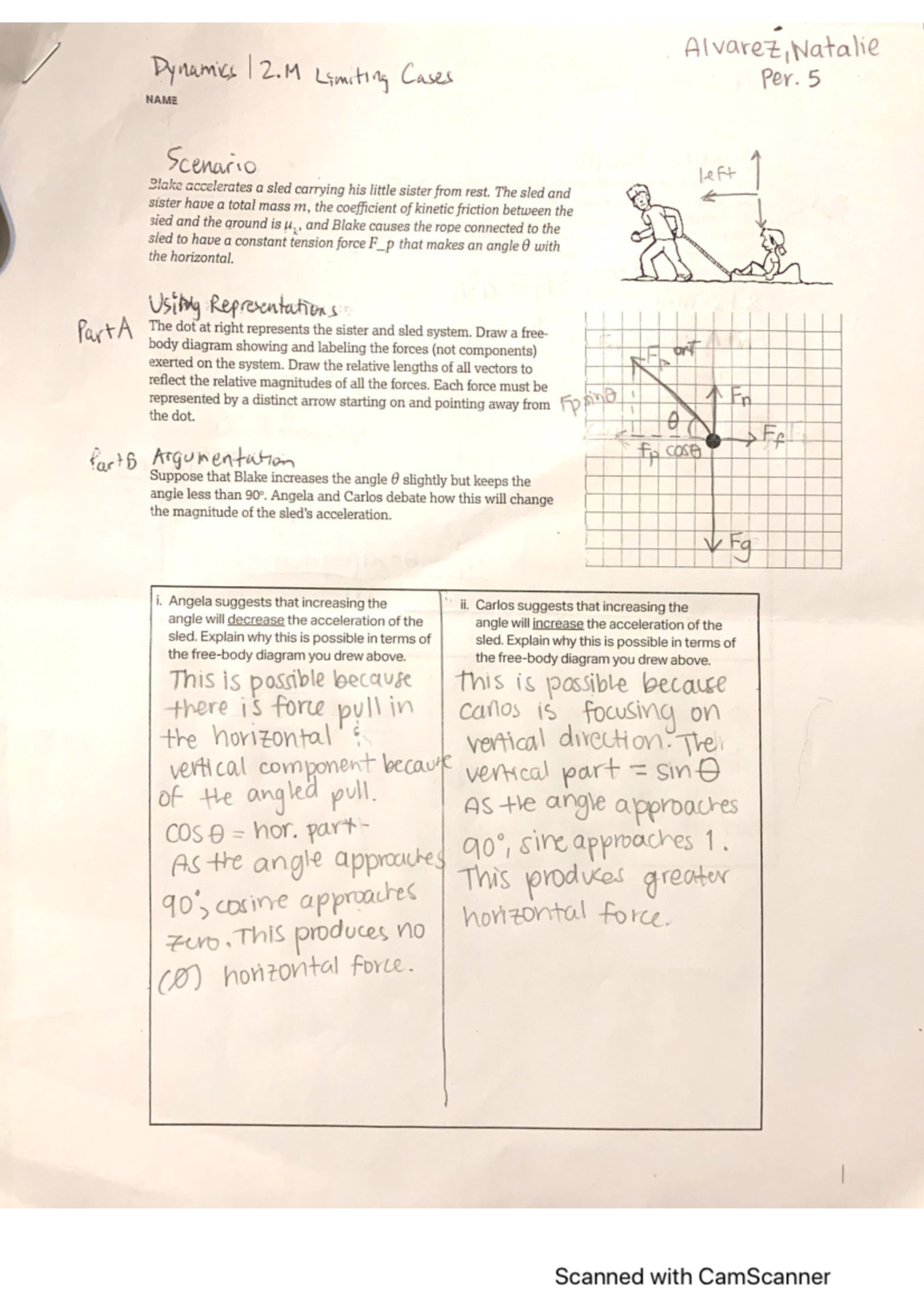
Take a moment to reason through this yourself.

Limit 1: $θ \to 0^{\circ}$ : The person pulls horizontally. All the pulling force contributes to the horizontal motion (minus friction). The vertical normal force is simply $F_{N} = F_{g}$ .
Limit 2: $θ \to 9 0^{\circ}$ : The person pulls straight up. The horizontal component of the pulling force, $F_{p} cos θ$ , goes to zero. Therefore, there is no force to overcome friction and cause horizontal acceleration. The sled doesn't move horizontally.

This simple thought experiment, analyzing the behavior at the boundaries of the parameter $θ$ , gives us a clear picture of the function a(\theta). This is the essence of using limiting cases.

The following reading provides a formal introduction to this strategy, along with others you should keep in mind.

Strategies for Solving Problems

The textbook 'Introduction to Classical Mechanics' by David Morin provides an excellent discussion on problem-solving strategies. We will focus on the sections that introduce the concepts of checking units and limiting cases.

Please read pages I-1 to I-5. Start at the beginning of the chapter and stop before Section 1.3 'Approximations, limiting cases'. Pay close attention to the general strategies listed and the detailed explanation of dimensional analysis. While our main focus today is on limits, dimensional analysis is a closely related tool for guessing and checking the form of physical equations.

2. The Mathematical Toolkit for Approximations

To analyze limiting cases quantitatively, we need mathematical tools that allow us to approximate complex functions when a variable is very small. For a physicist, the most indispensable of these are the Taylor series and the binomial theorem. Given your background in mathematics, you are likely familiar with these; here, our focus is on their strategic application to physical problems.

Problem Solving I: Mathematical Techniques

The handout 'Problem Solving I: Mathematical Techniques' by Kevin Zhou, written for Physics Olympiad training, provides a concise, physics-oriented summary of the essential approximation techniques.

Please read the sections 'Approximations' (starting on page 16) and 'Binomial Theorem' (page 19). You can stop before Example 11: Birthday Paradox on page 21. Focus on understanding how the Taylor series for exp(x), sin(x), cos(x), and 1/(1-x) are used. Pay special attention to the binomial theorem, (1 + x)^n ≈ 1 + nx for small x, as it is one of the most frequently used approximations in physics.

The key approximations to commit to memory are, for a small dimensionless quantity $ϵ ≪ 1$ :

Sine: $sin (ϵ) \approx ϵ$
Cosine: $cos (ϵ) \approx 1 - \frac{ϵ ^{2}}{2}$
Exponential: $e^{ϵ} \approx 1 + ϵ$
Binomial: $(1 + ϵ)^{n} \approx 1 + n ϵ$

A crucial point, emphasized in Morin's text, is that it only makes sense to talk about a quantity being "small" or "large" if it is dimensionless. An expression like t = 0.01s is not inherently small. But if a problem has a characteristic time τ = 1s, then the dimensionless ratio t/τ = 0.01 is small, and approximations are justified.

3. Applying the Techniques

Now let's see how these ideas—the philosophy of limits and the mathematics of approximation—come together to solve and verify kinematics problems.

Case Study 1: Verifying a Complex Formula

Imagine you've solved a difficult problem and arrived at a complicated answer. How do you check it?

Strategies for Solving Problems

Let's return to Morin's chapter. He provides an excellent worked example of using approximations to check the validity of the equations for motion with air resistance.

Please read Section 1.3, 'Approximations, limiting cases' (pages I-6 to I-9). Focus on Example 1 (Dropped ball). Observe how the complex expressions for v(t) and y(t) are analyzed in the limit of small t. Notice that 'small t' really means the dimensionless quantity αt << 1. The derivation shows how using the Taylor expansion e^{-x} ≈ 1 - x + x²/2 reduces the complex formulas to the familiar free-fall equations v(t) ≈ -gt and y(t) ≈ h - gt²/2. This should give you great confidence that the original formulas are correct.

This process of reducing a complex, general formula to a known, simpler case in a specific limit is one of the most satisfying "sanity checks" in physics.

Test your understanding!

Let's apply this verification technique. A person throws a ball with speed $v$ from the edge of a cliff of height $h$ . After a long derivation, you are presented with several possible formulas for the maximum horizontal range. Which of the following is the only plausible one? Use limiting cases to decide.

$\frac{g h ^{2}}{v ^{2}}, \frac{v ^{2}}{g}, \frac{v ^{2} h}{g}, \frac{v ^{2}}{g} 1 + \frac{2 g h}{v ^{2}}, \frac{v ^{2}}{g} (1 + \frac{2 g h}{v ^{2}})$

Hint: Consider two simple limits:

What happens when the cliff height $h = 0$ ? What is the standard formula for maximum range on level ground?
What happens if the launch speed $v$ is extremely large for a fixed $h$ ? How should the range behave?

Show answer

Let's test the options against the limiting cases.

Limit $h \to 0$ : The cliff disappears, and we have projectile motion on level ground. We know from Module 4 that the maximum range in this case is $R = v^{2} / g$ .
- $g h^{2} / v^{2} \to 0$ . Incorrect.
- $v^{2} / g \to v^{2} / g$ . Possible, but it implies range doesn't depend on $h$ at all, which is wrong.
- $v^{2} h / g \to 0$ . Incorrect.
- $\frac{v ^{2}}{g} 1 + \frac{2 g h}{v ^{2}} \to \frac{v ^{2}}{g} 1 = \frac{v ^{2}}{g}$ . Correct behavior.
- $\frac{v ^{2}}{g} (1 + \frac{2 g h}{v ^{2}}) \to \frac{v ^{2}}{g} (1) = \frac{v ^{2}}{g}$ . Correct behavior.
We are left with two candidates. Now let's consider the limit of small height, $h ≪ v^{2} / g$ . We can use the binomial approximation $1 + x \approx 1 + x /2$ .
- Candidate 1: $\frac{v ^{2}}{g} 1 + \frac{2 g h}{v ^{2}} \approx \frac{v ^{2}}{g} (1 + \frac{1}{2} \frac{2 g h}{v ^{2}}) = \frac{v ^{2}}{g} + h$ .
- Candidate 2: $\frac{v ^{2}}{g} (1 + \frac{2 g h}{v ^{2}}) = \frac{v ^{2}}{g} + 2 h$ .
The range is the base range $v^{2} / g$ plus some extra distance gained from the fall. For a very small height drop $h$ , the trajectory is almost symmetric. The optimal launch angle is close to 45°. At this angle, the trajectory is falling at 45° at the same height as the launch point. Geometrically, a small drop of $h$ vertically corresponds to a small extra horizontal distance of $h$ . Therefore, the expression that approximates to $\frac{v ^{2}}{g} + h$ is the more physically plausible one.

The correct formula is $\frac{v ^{2}}{g} 1 + \frac{2 g h}{v ^{2}}$ . This is discussed in problem 27 of the Zhou handout and problem 1.6 of the Morin handout.

Case Study 2: Deriving a Formula with Limits

Amazingly, you can sometimes work backwards and derive a formula by combining dimensional analysis with limiting cases.

Problem Solving I: Mathematical Techniques

Kevin Zhou's handout demonstrates this powerful synthesis by re-deriving the formula for projectile range.

Please read Section 4, 'Limiting Cases', on page 29, focusing on Example 13. Notice the rigorous chain of logic: Dimensional Analysis: The range R must depend on v and g, so R must be proportional to v²/g. Limiting Cases: The range must be zero for launch angles θ = 0 and θ = π/2. Synthesis: The simplest trigonometric function that is zero at 0 and π/2 (corresponding to 2θ=π) is sin(2θ). Approximation: To fix the constant of proportionality, check the θ << 1 limit using sin(2θ) ≈ 2θ, which confirms the constant is 1.

This approach beautifully blends physical reasoning with mathematical constraints to construct an answer from first principles, which aligns perfectly with your goal of a deeper, more fundamental understanding.

Conclusion

Today we've added a crucial technique to your problem-solving toolkit. While you have the mathematical prowess for complex derivations, the ability to step back and analyze a problem through the lens of its limiting behaviors is a hallmark of a mature physicist. It's a way to guide your intuition, check your work, and extract the core physics from a problem.

Key Takeaways:

Limiting cases are a tool for verification and intuition. By testing a formula in extreme (but simple) scenarios, you can quickly validate your work and understand the roles of different parameters.
Approximations are the mathematical engine for analyzing limits. The Taylor series for basic functions and the binomial theorem are essential for simplifying expressions when a dimensionless parameter is small.
The combination of dimensional analysis, limiting cases, and approximations can be a powerful method for deriving physical formulas from scratch.

Preview of the Next Lesson:

This is the final lesson in our module on advanced techniques, and the penultimate lesson of the course. You have mastered optimization with calculus, simplification through symmetry, and now analysis via approximations. In our next lesson, we will put it all together. You will be challenged to solve a capstone Olympiad-level problem requiring a creative synthesis of multiple kinematics concepts. This will be an opportunity to apply everything you have learned to tackle a problem that is both complex and rich with physical insight.

Recommended resources