Customer 360: Merging Data Sources

1. Relational Data: The "Why" Behind Merging

In the real world, data is almost never stored in a single giant table. Instead, it's organized into multiple, related tables. For example, a retailer might have:

• A transactions table (what was bought)
• A customers table (who bought it)
• A products table (details about the items)

This collection of related tables is called relational data. The power comes from the relations between them. To connect them, we use keys.

To understand these core concepts, please read the following sections from a lesson on relational data.

As you read, you'll see that a primary key uniquely identifies each row in its own table (e.g., CustomerID in a customer table), while a foreign key is a key from another table used to refer to it (e.g., CustomerID in the transactions table). This key-based structure is what allows us to merge our data accurately.

2. The Anatomy of a Merge

In pandas, the most powerful and flexible tool for this job is the .merge() function. Merging, or joining, combines dataframes side-by-side based on the values in one or more common columns (our keys).

There are four main types of joins, each answering a slightly different business question. The visual metaphors of Venn diagrams are extremely helpful here.

The four main types are:

• Inner Join: Returns only the rows that have matching keys in both DataFrames.
  • Business Question: "Show me the customers for whom I have both transaction data and demographic data."
• Left Join: Returns all rows from the left DataFrame, and the matched rows from the right DataFrame. If there is no match, the columns from the right DataFrame will be filled with NaN.
  • Business Question: "Show me all the customers who have made a purchase, and add their demographic information if we have it."
• Right Join: The reverse of a left join. It returns all rows from the right DataFrame.
  • Business Question: "Show me all the customers in our demographics file, and add their purchase history if they have any."
• Outer Join (or Full Join): Returns all rows from both DataFrames, filling in NaN where matches don't exist.
  • Business Question: "Show me a complete list of everyone, whether they're in our transaction logs, our demographics file, or both."

For a dynamic explanation of these concepts with code, the following video is an excellent resource.

3. Merging in Practice: Building the Customer View

Now, let's apply these concepts to our customer analytics goal. Imagine you have two DataFrames:

1. customer_summary_df: The table you created in the last lesson, with CustomerID, Recency, Frequency, and Monetary.
2. demographics_df: A table with CustomerID, Age, Income_Bracket, and Gender.

Our goal is to create a single, unified table. Based on the business questions we discussed, a left join is usually the most appropriate choice. We want to start with our primary list of customers (those who have transacted) and enrich it with additional information.

# The left DataFrame is our primary source of truth
# The right DataFrame provides the enrichment data
enriched_customer_df = customer_summary_df.merge(
    demographics_df,      # The right DataFrame
    how='left',           # The type of join
    on='CustomerID'       # The key column to join on
)

This simple line of code is incredibly powerful. You now have a single DataFrame where you can analyze relationships between behavior (frequency, monetary) and demographics (age, income).

Handling Common Scenarios

1. Keys with Different Names

What if the customer identifier is CustomerID in one table but customer_ID in another? The on parameter won't work. Instead, you use left_on and right_on.

enriched_df = customer_summary_df.merge(
    demographics_df,
    how='left',
    left_on='CustomerID',   # Key in the left DataFrame
    right_on='customer_ID'  # Key in the right DataFrame
)

This will result in two key columns in the output (CustomerID and customer_ID), so you'll typically drop one after the merge.

2. Verifying Your Merge

How do you know the merge worked as expected? What if you want to know how many customers from your transaction summary didn't have a match in the demographics file? The indicator=True argument is your best friend.

Using the indicator lets you answer critical business questions like, "Of our 10,000 active customers, how many are we missing demographic information for?" You can find this by simply filtering for rows where _merge == 'left_only'.

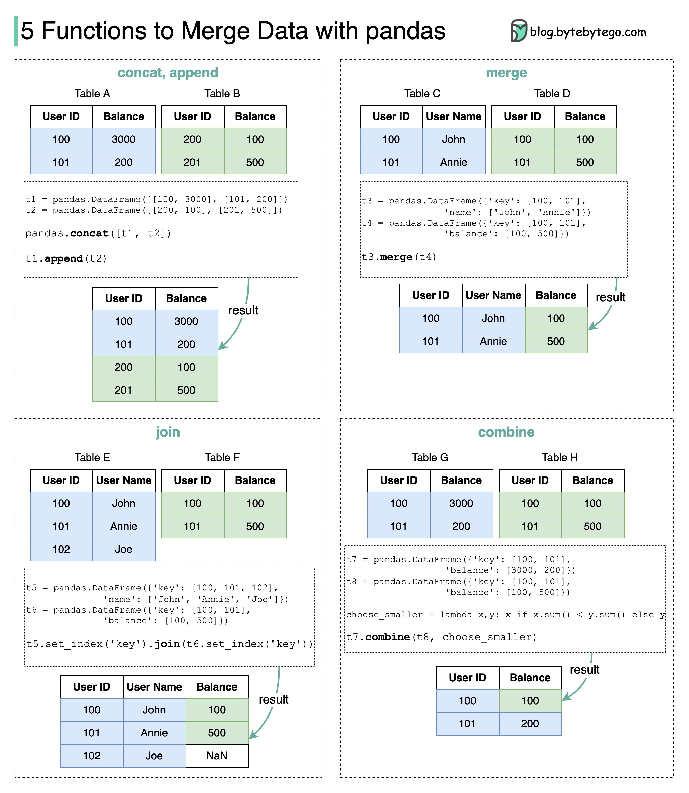
4. merge vs. join vs. concat

You may see join and concat used as well. It's important to know the difference:

• merge(): The most versatile function. Use this for combining DataFrames on common columns. It can do everything the other functions can and is more explicit. This should be your default choice.
• join(): A convenience method that joins DataFrames on their index. It's less flexible than .merge() but can be a quick shortcut if your DataFrames are already indexed by the key you want to join on.
• concat(): This function stacks DataFrames, either vertically (adding rows) or horizontally (adding columns). It does not use keys to align data; it aligns based on the index. You would use concat to combine transaction files from January and February, not to add demographic data to transactions.

The following case study provides a concise summary and a clear, step-by-step example of merging multiple files.

Conclusion

You have now learned how to break down data silos and create a unified view of your customers. This is a foundational skill that moves you from basic data manipulation to true customer analytics.

Key Takeaways:

• The Goal: To create a single customer view by combining multiple data sources (e.g., transactions, demographics).
• The Core Concept: Relational data is linked by keys (primary and foreign).
• The Main Tool: pd.merge() is the most flexible and powerful function for this task.
• Critical Parameters:
  • how: Determines the logic of the merge (left, right, inner, outer). left is often the most useful for enriching a primary dataset.
  • on, left_on, right_on: Specify the key(s) for the merge.
  • indicator=True: A powerful tool for auditing your merge and gaining business insights about data completeness.

In our next lesson, we will put this newly created dataset to work. We'll begin our journey into Exploratory Analysis of Customer Behavior, where you will learn to formulate and answer business questions using the comprehensive customer view you now know how to build.