Hello! Welcome to your next lesson in the Mathematics Mastery Sprint.
In our last lesson, we learned how to calculate and interpret measures of central tendency (mean, median, mode) and spread (range, IQR) from lists and tables, including grouped frequency tables. You became familiar with using midpoints to estimate the mean for grouped data.
Today, we'll build directly on that foundation. We will learn how to visually represent grouped continuous data using a powerful statistical diagram that frequently appears on Paper 4: the histogram. Your specific learning outcome is to construct and interpret histograms with unequal class widths.
This is a key topic that often trips students up, but it's very manageable once you grasp one central concept. Mastering this will help you tackle a type of question you've found challenging in the past: graphs.
1. Why Histograms are Different from Bar Charts
You're used to bar charts, where the height of each bar represents the frequency. This works when all the categories (or bars) have the same width. But what happens when you have grouped data with unequal class widths, like we saw in the last lesson?
Consider this table:
| Time (t minutes) | Frequency | Class Width |
|---|---|---|
| 0 < t ≤ 10 | 20 | 10 |
| 10 < t ≤ 30 | 40 | 20 |
If we drew a bar chart, the second group (frequency 40) would have a bar twice as high as the first (frequency 20). However, the second group's data is spread over an interval that is twice as wide. This is misleading. A histogram solves this problem with one fundamental rule:
In a histogram, the AREA of the bar represents the frequency, not the height.
This means we need a new value for the y-axis that ensures the area relationship holds true. This value is called Frequency Density.
2. Constructing a Histogram: The Role of Frequency Density
Since Area = Height × Width, and we want Frequency = Area, it follows that:Frequency = Height × Class Width
Rearranging this gives us the formula for the height of each bar:
Let's watch a video that explains this core concept and then walks through the process of drawing a histogram from a table.
Histograms - How to Draw and Interpret a Histogram | Grade 7-9 Playlist | GCSE Maths Tutor
This video from The GCSE Maths Tutor provides an excellent analogy for understanding frequency density and then gives a clear, step-by-step guide to constructing a histogram.
Watch the following two segments: The Core Concept (00:53 - 05:32): Pay close attention to the rectangle analogy. This is the key to understanding why we use frequency density. The video will formalise this into the main formula you need. Worked Example (05:32 - 09:25): Follow along as a histogram is drawn from a frequency table. Notice the three steps: calculate class widths, calculate frequency densities, then draw the bars with the correct width and height (frequency density).
Here is a static image that summarises the process you just watched. It's a useful reference.

Common Pitfalls
Before you practice, let's highlight some common errors students make. Being aware of these will help you avoid them.
Histograms - GCSE Maths - Steps, Examples & Worksheet
This text from Third Space Learning outlines some very common mistakes. Read this section carefully to pre-emptively fix potential errors in your own work.
Read the section titled 'Common misconceptions'. Pay particular attention to the difference between frequency and frequency density, and how the area (not height) represents frequency.
Test your understanding! (Past Paper Question)
This question tests the core principle of frequency density in a typical exam format. You don't need to draw anything, just calculate.
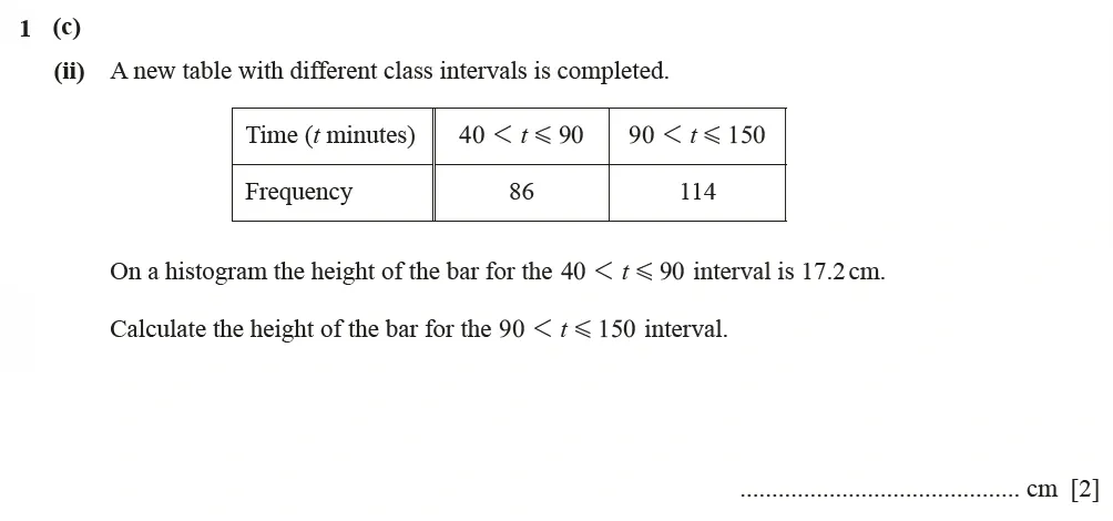
Hint: The height is proportional to the frequency density, but not always equal to it. There might be a scaling factor.
Show answer
-
Analyse the first bar (the one we know everything about):
- Frequency () = 86
- Class Width () = 90 - 40 = 50
- Frequency Density () =
-
Find the relationship between Frequency Density and Height:
- We calculated , but the question states the height is 17.2 cm.
- This means
Height = k × Frequency Density, wherekis a scaling factor. - . Solving for
k, we find thatk = 10. - So, for this histogram, the rule is: Height = 10 × Frequency Density.
-
Apply the rule to the second bar:
- Frequency () = 114
- Class Width () = 150 - 90 = 60
- Frequency Density () =
-
Calculate the final height:
- Height of the second bar = cm.
Final Answer: 19 cm.
3. Interpreting Histograms
Now let's reverse the process. Interpreting histograms involves reading information from the graph to calculate frequencies or complete a table. This often means using the core formula rearranged:
Method 1: Using the Frequency Density Scale
The most common task is finding the frequency of one or more bars. You read the height (Frequency Density) from the y-axis and the width from the x-axis, then multiply them. Watch this example where a partially drawn histogram is used to complete a table.
Histograms - How to Draw and Interpret a Histogram | Grade 7-9 Playlist | GCSE Maths Tutor
This segment from The GCSE Maths Tutor shows how to tackle a common exam question: completing a histogram and a frequency table when some information is missing.
Watch from 14:38 to 19:52. The key first step is to use a bar for which you have information both in the table and on the graph. This allows you to figure out the scale on the frequency density axis. Once the scale is known, you can find all the other missing values.
Another common interpretation task is to estimate the number of items within part of a bar. For example, estimating how many animals weigh more than 80 kg when the bar covers the 75-85 kg range.
Histograms - How to Draw and Interpret a Histogram | Grade 7-9 Playlist | GCSE Maths Tutor
This final clip demonstrates how to estimate frequencies for intervals that fall inside a single bar. This is a higher-level interpretation skill.
Watch from 24:13 to 28:29. The key assumption here is that the data is evenly distributed throughout the interval. If you need to find the frequency for half the interval, you take half the area (i.e., half the frequency) of that bar.
Method 2: The "Counting Blocks" Strategy (An alternative approach)
Sometimes, a question gives you the total frequency for the entire histogram but provides no scale on the y-axis. In these cases, you can't calculate frequency density directly. This is where a different method is needed, which aligns with your goal of learning more efficient problem-solving strategies.
9-1 GCSE Maths - Histograms - Unequal Class Intervals - Frequency Density -Higher
This video from ukmathsteacher demonstrates the 'counting blocks' method. It's a powerful alternative for specific types of exam questions.
Watch from 16:33 to 21:13. The strategy is: Calculate the total area of the histogram in 'small squares' or 'blocks'. Find how much frequency one 'block' is worth by dividing the total frequency by the total number of blocks. Use this value to find the frequency of any other area you are interested in.
This method is an excellent example of choosing the right tool for the job, rather than trying to force a single method onto every problem.
Conclusion
You've done an excellent job covering the essential skills for histograms. These questions are a great way to pick up marks on Paper 4 if you are methodical and careful with your calculations.
Key Takeaways:
- The Golden Rule: In a histogram, Area = Frequency.
- Constructing: To draw a histogram, you must first calculate the Frequency Density for each class and use this for the bar's height. The formula is .
- Interpreting: To find the frequency from a bar, you use the reverse formula: .
- Estimation: To estimate the frequency for a part of a bar, you assume the data is evenly spread. For example, the frequency in one-quarter of a class interval is one-quarter of that bar's total frequency.
- Problem-Solving: Always check if the y-axis is scaled. If it isn't, and you are given the total frequency, the "counting blocks" method is an effective strategy.
Preview of the Next Lesson:
We have now concluded the Probability and Statistics module. In the next lesson, we will begin a new topic: Geometric Transformations and Vectors. We will start by learning how to describe and perform single transformations like rotations, reflections, translations, and enlargements.