Bootstrapping Spot Rates in Python

Introduction

In our last lesson, you mastered the mathematical derivation of a spot rate curve from an idealized par-yield curve. This gave you a solid grasp of the recursive logic at the heart of bootstrapping: using known, shorter-term spot rates to solve for the next, longer-term spot rate in the sequence.

Today, we will translate that theoretical understanding into practice. Your objective is to implement the bootstrapping algorithm in Python to construct a spot rate curve not from a perfect par curve, but from real market data—a collection of bonds with varying coupons, maturities, and market prices. This will equip you with a core skill for practical fixed-income analysis.

1. The Bootstrapping Process with Market Bonds

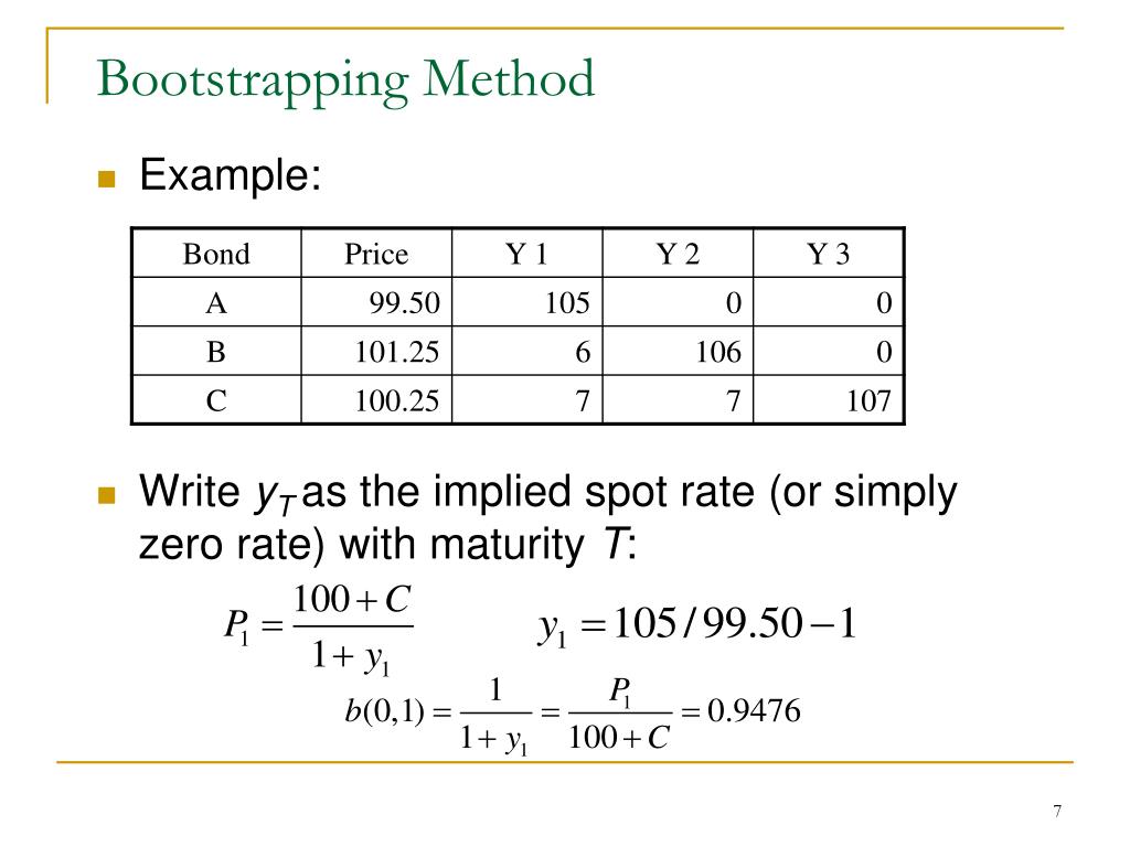
The fundamental logic of bootstrapping remains unchanged when moving from a theoretical par curve to a set of actual market bonds. However, instead of assuming all bonds are priced at par (100), we now use their observable market prices.

The process involves selecting a set of bonds of the same credit quality (e.g., government bonds) with staggered maturities. We then extract the spot rates one by one, moving from the shortest maturity to the longest. The video below provides an excellent high-level overview of this iterative process.

As the video shows, the core task for each bond is to solve for the one unknown spot rate corresponding to its final cash flow, using its market price and the spot rates we've already derived from shorter-maturity bonds.

2. The Bootstrapping Algorithm

Let's formalize the algorithm for a bond with $T$ periods to maturity and a market price $P$. Assuming semi-annual payments (so $k=2$ payments per year) and a face value of $FV$, its price is the sum of its discounted cash flows:

At each step, we have a bond whose final cash flow corresponds to the spot rate we want to find. All prior spot rates are known. We can rearrange the equation to solve for the unknown spot rate, $s_T$, where $T$ is the number of periods:

The term ${\sum }_{t=1}^{T-1}\dots$ is the present value of all coupons before maturity, discounted using the spot rates we've already calculated. Let's call this $P{V}_{coupons}$. The equation simplifies to:

Solving for $s_T$ gives us the formula we'll implement:

This is the engine of our Python implementation.

3. A Practical Implementation Guide

The following article provides a superb, in-depth guide to implementing this algorithm using real US Treasury bond data. It covers not only the core formula but also practical considerations like data collection.

4. Implementing the Bootstrapper in Python

Now, let's synthesize this logic into a complete Python function. We will take a list of bonds, where each bond is represented by its maturity, market price, and coupon rate. The function will return the bootstrapped spot curve.

For this example, we'll use a simplified set of semi-annual coupon bonds with a face value of 100. The input data is sorted by maturity.

import math

def bootstrap_spot_curve(bonds):
    """
    Bootstraps a spot rate curve from a list of bonds.

    Args:
        bonds (list of dicts): A list of bond data, where each dict has
                              'maturity' (in years), 'price' (market price),
                              and 'coupon' (annual coupon rate).
                              Bonds must be sorted by maturity.

    Returns:
        dict: A dictionary mapping maturities to their corresponding spot rates.
    """
    spot_curve = {}
    face_value = 100.0
    
    for bond in bonds:
        maturity = bond['maturity']
        price = bond['price']
        coupon_rate = bond['coupon']
        



        # Calculate the semi-annual coupon payment
        coupon_payment = face_value * coupon_rate / 2.0
        



        # Calculate the number of periods (semi-annual)
        num_periods = int(maturity * 2)
        



        # --- Calculate PV of known coupons ---
        pv_coupons = 0.0
        for t in range(1, num_periods):



            # t/2 gives the maturity in years for the t-th period
            # For example, for a 2-year bond, period t=1 is at 0.5 years, t=2 is at 1.0 year etc.
            t_maturity = t / 2.0
            if t_maturity in spot_curve:
                spot_rate = spot_curve[t_maturity]



                # Discount the coupon payment for period t
                pv_coupons += coupon_payment / ((1 + spot_rate / 2.0) ** t)
        



        # --- Solve for the unknown spot rate ---
        # The numerator is the final cash flow (last coupon + face value)
        final_cash_flow = face_value + coupon_payment
        



        # The denominator is the bond's price minus the PV of intermediate coupons
        denominator = price - pv_coupons
        



        # This is the direct implementation of our formula
        # ( (final_cf / denominator) ^ (1/T) ) - 1
        semi_annual_spot = (final_cash_flow / denominator) ** (1 / num_periods) - 1
        



        # Annualize the spot rate
        annual_spot_rate = semi_annual_spot * 2
        
        spot_curve[maturity] = annual_spot_rate
        
    return spot_curve


```grasp
{
  "type": "exercise",
  "id": "a8ef3717-30e4-449b-b932-075e828fcd20"
}