Bootstrapping Bonds with Variable Coupon Frequencies

Introduction

In our last lesson, you successfully implemented a Python bootstrapping algorithm, turning a set of market bond prices into a discrete spot rate curve. This was a significant step, but our implementation relied on a simplifying assumption: that all bonds pay coupons semi-annually. In practice, the bond market is a diverse ecosystem with instruments featuring annual, semi-annual, quarterly, or even other payment frequencies.

Today, we will generalize our bootstrapping logic to handle this complexity. Your objective is to adjust the algorithm to correctly process a mix of bonds with varying coupon frequencies. This enhancement will transform our Python function from a textbook example into a more robust and practical tool, a process that should feel familiar given your background in building flexible data science models.

1. Generalizing the Discounting Formula

The foundation of our adjustment lies in parameterizing the coupon frequency. Let's define a parameter, $f$ , as the number of coupon payments per year (e.g., $f = 1$ for annual, $f = 2$ for semi-annual, $f = 4$ for quarterly).

Recall the semi-annual bond pricing formula, where $M$ is the maturity in years:

P = t = 1 \sum 2 \cdot M \frac{C /2}{( 1 + \frac{s _{ann, t /2}}{2} ) ^{t}}

Here, the number of periods is $2 \cdot M$ , the coupon per period is $C /2$ , and the periodic discount rate is the annualized spot rate $s_{ann}$ divided by 2.

By substituting our frequency parameter $f$ , we arrive at a generalized formula that works for any payment frequency:

P = t = 1 \sum f \cdot M \frac{C / f}{( 1 + \frac{s _{ann, t / f}}{f} ) ^{t}}

This generalized formula is the key to handling different bond structures. Each component is now expressed in terms of $f$ :

Number of periods: $f \cdot M$
Coupon payment per period: $C / f$
Periodic spot rate: $s_{ann} / f$

This approach of explicitly defining frequency allows us to build a more versatile pricing engine.

Computing Risk Free Rates and Excess Returns Part 2

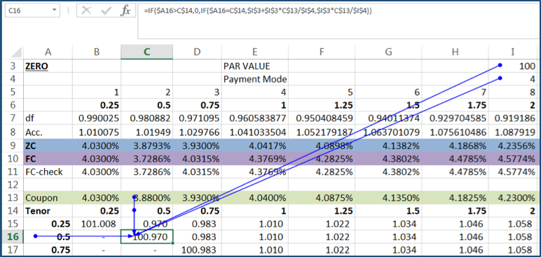
Let's revisit the LSEG article we used in the last lesson. It introduces a similar concept, which will help connect to what you already know.

Please review the first section, "YTM of Coupon Paying Bonds," focusing on the introduction of the variables f_{\text{acf}} and f_{\text{acpf}}. Notice that the author uses f_{\text{acf}} = 0.5 for semi-annual compounding. This is the period length in years. Our parameter, f, represents the frequency per year. The two are inversely related (f = 1/f_{\text{acf}}). Both approaches are valid, but using frequency (f=1, 2, 4) is often more intuitive when coding.

2. Adapting the Bootstrapping Algorithm

The core challenge in adapting our algorithm is to ensure it can handle a list of bonds where each bond may have a different frequency. This means the frequency, $f$ , must be an attribute of each individual bond, not a single setting for the entire calculation.

The documentation for the QuantBondCurves R package highlights this exact requirement for a robust implementation.

QuantBondCurves - CRAN

This vignette describes an industry-standard implementation for curve calibration.

Read the section on "Curve Calibration" and focus on the description of the freq parameter. The text notes: "freq parameter can be provided as either a single value that applies to all input assets, or as a vector in which each element corresponds to a specific asset." This is precisely the capability we are building into our Python function.

With this in mind, let's generalize the bootstrapping formula we derived in the previous lesson. The original formula for the annualized spot rate was:

s_{ann, M} = 2 \times [(\frac{F V + C /2}{P - P V _{co u p o n s}})^{1/ (2 \cdot M)} - 1]

Using our frequency parameter $f$ for the bond being solved, the generalized formula becomes:

s_{ann, M} = f \times [(\frac{F V + C / f}{P - P V _{co u p o n s}})^{1/ (f \cdot M)} - 1]

The calculation of $P V_{co u p o n s}$ also needs to be updated. When calculating the present value of the intermediate coupons for a bond with frequency $f$ , each coupon must be discounted using a periodic spot rate derived for that specific cash flow date, but using the same frequency $f$ . That is, the periodic rate for a coupon at time $t / f$ is $s_{ann, t / f} / f$ .

3. Updating the Python Implementation

Now we will modify the bootstrap_spot_curve function from our previous lesson. The key changes are:

Each bond in our input list will now have a 'freq' attribute.
The calculations for coupon payments, number of periods, and discounting will be generalized to use this freq value.
The final annualization step will also use the bond's specific frequency.

Below is the updated code. Pay close attention to how f is used throughout the calculations.

import math

def bootstrap_spot_curve_flexible_freq(bonds):
    """
    Bootstraps a spot rate curve from a list of bonds with varying frequencies.

    Args:
        bonds (list of dicts): A list of bond data, where each dict has
                              'maturity' (in years), 'price' (market price),
                              'coupon' (annual coupon rate), and 'freq' (payments per year).
                              Bonds must be sorted by maturity.

    Returns:
        dict: A dictionary mapping maturities to their corresponding annualized spot rates.
    """
    spot_curve = {}
    face_value = 100.0
    



    # We assume the input bonds are sorted by maturity to enable bootstrapping.
    for bond in bonds:
        maturity = bond['maturity']
        price = bond['price']
        coupon_rate = bond['coupon']
        f = bond['freq'] # Get the frequency for the current bond
        



        # Handle zero-coupon bonds as a special case (their YTM is the spot rate)
        if coupon_rate == 0.0:



            # P = FV / (1 + s/f)^(f*M) => s = f * ( (FV/P)^(1/(f*M)) - 1 )
            # For ZCBs, f*M is usually 1 period, but we use the full formula for generality.
            annual_spot_rate = f * (((face_value / price)**(1 / (f * maturity))) - 1)
            spot_curve[maturity] = annual_spot_rate
            continue




        # For coupon bonds:
        # 1. Generalize coupon payment and number of periods
        coupon_payment = face_value * coupon_rate / f
        num_periods = int(maturity * f)
        



        # 2. Calculate PV of known intermediate coupons
        pv_coupons = 0.0



        # Loop through the periods of the *current* bond
        for t in range(1, num_periods):



            # The maturity corresponding to period t
            t_maturity = t / f
            



            # This is a simplification. In reality, we need a spot rate for t_maturity.
            # A robust implementation would require interpolation if the exact spot
            # rate isn't in the curve, which we will cover in the next lesson.
            # For today, we assume our bond set provides the necessary spot rates.
            if t_maturity in spot_curve:



                # Get the annualized spot rate from the curve
                annual_spot_rate = spot_curve[t_maturity]



                # De-annualize it using the current bond's frequency
                periodic_spot_rate = annual_spot_rate / f
                
                pv_coupons += coupon_payment / ((1 + periodic_spot_rate) ** t)
        



        # 3. Solve for the unknown spot rate using the generalized formula
        final_cash_flow = face_value + coupon_payment
        denominator = price - pv_coupons
        



        # This solves for the periodic spot rate
        periodic_spot = (final_cash_flow / denominator) ** (1 / num_periods) - 1
        



        # 4. Annualize the result using the current bond's frequency
        annual_spot_rate = periodic_spot * f
        
        spot_curve[maturity] = annual_spot_rate
        
    return spot_curve




# --- Example Usage with Mixed Frequencies ---
# We need a set of bonds where maturities allow sequential bootstrapping.
market_bonds_mixed = [
    {'maturity': 0.5, 'coupon': 0.00, 'price': 99.502, 'freq': 2},  # 6-mo ZCB (yields 1.0%)
    {'maturity': 1.0, 'coupon': 0.012, 'price': 99.805, 'freq': 1}, # 1-yr ANNUAL bond
    {'maturity': 1.5, 'coupon': 0.015, 'price': 99.558, 'freq': 2}, # 1.5-yr SEMI-ANNUAL bond
    {'maturity': 2.0, 'coupon': 0.020, 'price': 99.230, 'freq': 4}  # 2-yr QUARTERLY bond
]




# Build the spot curve
bootstrapped_curve_mixed = bootstrap_spot_curve_flexible_freq(market_bonds_mixed)




# Print the results
print("Bootstrapped Spot Curve (Mixed Frequencies):")
for maturity, rate in bootstrapped_curve_mixed.items():
    print(f"Maturity: {maturity:<4} years | Spot Rate: {rate:.4%}")

Code Walkthrough with an Example

Let's trace the calculation for the final bond in our list: the 2-year quarterly bond ( $f = 4$ ).

Initialization: The code retrieves the bond's properties: maturity=2.0, coupon=0.02, price=99.230, and f=4.
PV of Known Coupons: The loop for pv_coupons runs for t from 1 to 7 (since num_periods is $2 \times 4 = 8$ ).
- t=1 (0.25 years): No spot rate at 0.25 years is in our curve. Our simple code skips this, but a real system would need to interpolate (our topic for next lesson!). Let's assume for now we have rates for all prior coupon dates.
- t=2 (0.5 years): t_maturity is 0.5. The code finds s_0.5 = 1.000% in the spot_curve. It calculates a quarterly-compounded periodic rate: 1.000% / 4 = 0.25%. The coupon of $0.50 ( $100 \times 0.02/4$ ) is discounted: $\frac{0.50}{( 1 + 0.0025 ) ^{2}}$ .
- t=4 (1.0 years): t_maturity is 1.0. It finds s_1.0 in the curve. It de-annualizes this rate by 4 and discounts the coupon over 4 periods.
- ...This continues for all 7 intermediate coupons.
Solve for Final Spot Rate: After summing the present values of the first 7 coupons into pv_coupons, the code solves for the final 2-year spot rate using our generalized formula, annualizing the result by multiplying the periodic rate by 4.

This example demonstrates the flexibility of the new function. It correctly de-annualizes known spot rates based on the frequency of the bond being priced, a crucial detail for an accurate implementation.

Excel Bootstrapping for Zero-Coupon Yield Curve — This spreadsheet illustrates the iterative nature of bootstrapping. Notice the tenors (0.25, 0.50, etc.), implying instruments with different payment schedules are used. The calculation for each new discount factor ('df') relies on the previously computed ones, just as our Python code uses previously found spot rates to solve for the next.

Conclusion

You have now successfully generalized your bootstrapping algorithm, making it significantly more powerful and applicable to real-world market data. By parameterizing the coupon frequency, you've engineered a solution that can handle a diverse set of bonds within a single, unified framework.

Key Takeaways:

Parameterize Frequency: The key to handling varying bond structures is to introduce a frequency parameter, $f$ , and make it an attribute of each bond.
Generalize Formulas: All core calculations—coupon per period, number of periods, discounting, and annualization—must be expressed in terms of $f$ .
On-the-Fly (De-)Annualization: A robust spot curve should store consistent, annualized rates. The conversion to a periodic rate for discounting should happen dynamically within the calculation, using the frequency of the bond currently being priced.
Data Dependencies: Practical bootstrapping requires a carefully selected set of bonds where shorter-maturity instruments provide the spot rates needed to price longer-maturity ones.

Our bootstrapping algorithm now produces a discrete set of spot rates. But what if we need to price a bond with a cash flow at 1.75 years, and we only have spot rates for 1.5 and 2.0 years? In our next lesson, we will tackle this exact problem by exploring interpolation techniques to create a continuous yield curve from our discrete bootstrapped points.