Approximating Bond Price Changes with Modified Duration

From the Derivative to a Practical Approximation

The definition of Modified Duration involves the derivative $\frac{dP}{dy}$, which describes an infinitesimally small change. For practical purposes, we need to estimate the price change ($\Delta P$) for a discrete change in yield ($\Delta y$). We can do this by rearranging the definition of Modified Duration and replacing the differential terms with discrete changes:

Starting with:
$D_{\text{mod}}=-\frac{1}{P}\frac{dP}{dy}$

For small changes, we can approximate the derivative as a ratio of differences, $\frac{dP}{dy}\approx \frac{\Delta P}{\Delta y}$. Substituting this in gives:
$D_{\text{mod}}\approx -\frac{1}{P}\frac{\Delta P}{\Delta y}$

Now, we can solve for the percentage price change, $\frac{\Delta P}{P}$:

$\frac{\Delta P}{P}\approx -D_{\text{mod}}\cdot \Delta y$

This is the core formula for today's lesson. It states that the approximate percentage change in a bond's price is equal to its Modified Duration multiplied by the change in yield, with a negative sign to reflect the inverse relationship.

This approximation is mathematically equivalent to using the first-order term of a Taylor series expansion of the price function $P(y)$ around the initial yield $y_0$. Your background in mathematics will recognize this as a linear approximation, or a tangent line approximation, of a curve.

The following resource provides a formal and concise derivation starting from the Taylor expansion.

Applying the Formula: A Worked Example

Now let's see this formula in action. The following video provides a clear, step-by-step example of calculating the percentage price change for a bond given its Modified Duration and a hypothetical change in yield.

As the video demonstrates, if a bond has a Modified Duration of 4.43 and its yield increases by 1% (i.e., $\Delta y=+0.01$), the approximate price change is:

$\frac{\Delta P}{P}\approx -4.43\times 0.01=-0.0443$

This implies the bond's price will decrease by approximately 4.43%.

Understanding the Approximation Error

The key word in our discussion is "approximation." Because the true price-yield relationship is a curve, a linear approximation will inevitably have some error, especially as the change in yield becomes larger.

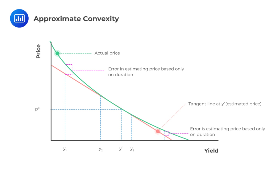
This error occurs because duration only captures the first-order (linear) effects. The curvature itself, which we will later quantify as convexity, means that:

• For a decrease in yield, the linear approximation underestimates the actual price increase.
• For an increase in yield, the linear approximation overestimates the actual price decrease.

The next video provides an excellent, practical demonstration of this concept. It compares the price change estimated using only duration to the exact price change calculated by re-pricing the bond at the new yield.

Python Implementation

Given your background, let's translate this directly into a Python function. The implementation is straightforward, directly reflecting the formula we've been using.

def estimate_price_change_pct(modified_duration: float, yield_change: float) -> float:
    """
    Approximates the percentage change in a bond's price using Modified Duration.

    Args:
        modified_duration (float): The bond's Modified Duration.
        yield_change (float): The change in yield (e.g., 0.01 for a 1% increase).

    Returns:
        float: The approximate percentage change in the bond's price.
    """
    return -modified_duration * yield_change




# --- Example Usage ---
# Using the example from the Edspira video (resource [LINK](https://www.youtube.com/watch?v=rdDfmlerTcI))
mod_d = 4.43
delta_y = 0.01  # A 1% increase in yield

estimated_pct_change = estimate_price_change_pct(mod_d, delta_y)

print(f"Bond with Modified Duration of {mod_d}:")
print(f"For a yield change of {delta_y*100:.2f}%, the estimated price change is {estimated_pct_change*100:.4f}%")




# --- Example of a yield decrease ---
delta_y_decrease = -0.005 # A 50 basis point (0.5%) decrease
estimated_pct_change_decrease = estimate_price_change_pct(mod_d, delta_y_decrease)
print(f"For a yield change of {delta_y_decrease*100:.2f}%, the estimated price change is {estimated_pct_change_decrease*100:.4f}%")

This simple function is a powerful first step in building a bond risk analytics toolkit. The Jupyter Notebook in the resources contains a more elaborate version that plots the exact price curve against the duration approximation, similar to the graph shown above. You can find the relevant code in the "Approximation" section, specifically the calculation for P_1.

Conclusion

Today we have put Modified Duration to work. We have established its practical application as a tool for estimating the percentage change in a bond's price for a small shift in interest rates.

Key Takeaways:

• The practical formula for price approximation is: $\frac{\Delta P}{P}\approx -D_{\text{mod}}\cdot \Delta y$.
• This is a linear approximation, mathematically equivalent to the first-order term of a Taylor series expansion of the price-yield function.
• Because the true price-yield relationship is convex, the duration approximation is most accurate for small yield changes and systematically underestimates gains and overestimates losses.

We've now seen the power of the first derivative. However, we've also clearly identified its limitation: the approximation error caused by the bond's convexity. In our next lesson, we will tackle this head-on by defining and deriving Convexity as the second derivative of the price-yield function, allowing us to build a far more accurate second-order approximation.