Introduction
Welcome to the next lesson in our exploration of the term structure of interest rates. In the previous session, we established the theoretical foundation for forward rates, deriving their relationship with spot rates from the crucial no-arbitrage principle. You learned that the equation mathematically links the spot and forward rate curves, ensuring they are internally consistent.
Today, we will transition from theory to practice. The objective of this lesson is to implement a Python function that computes a forward rate curve from a given spot rate curve. By the end of this lesson, you will have built another key component of our bond analytics toolkit, enabling you to extract market expectations of future rates directly from the zero-coupon yield curve.
1. Recapping the Forward Rate Calculation
Let's begin with a quick review of the core concept. The no-arbitrage argument implies that the return from investing in a long-term zero-coupon bond must be equivalent to the return from investing in a short-term bond and rolling the proceeds into a forward agreement.
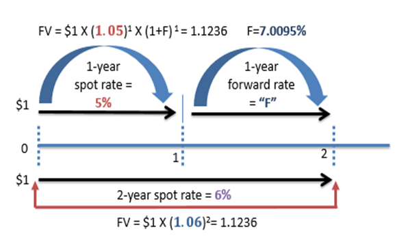
From the previous lesson, we derived the general formula for the forward rate annualized over the period :
where and are the spot rates for maturities and , respectively.
To build our forward curve, we will typically compute a series of one-year forward rates, such as the forward rate from year 1 to 2, from year 2 to 3, and so on. Let's specialize the general formula for a one-year forward rate starting at time , denoted . Here, and , so .
The formula simplifies to:
This equation will be the engine of our Python function. The following short video provides a numerical example of this exact calculation.
How to Calculate Spot Rates and Forward Rates in Bonds
This video from Ryan O'Connell, CFA, FRM, provides a clear, step-by-step numerical calculation of forward rates from spot rates.
Watch the entire video, paying close attention to the logic connecting the spot rates for different periods to the implied forward rates. Notice how the calculation for the year 1-to-2 forward rate and the year 2-to-3 forward rate directly applies the formula we just discussed.
2. Deriving the Forward Curve from a Spot Curve
With the formula for one-year forward rates established, let's walk through an example to solidify the process before we start coding. The following reading provides a clear set of spot rates and the resulting forward rates.
The Term Structure of Interest Rates, Spot Rates, and Yield to Maturity
This excerpt from a textbook by the University of Pennsylvania's Wharton School provides a worked example of calculating a forward curve.
Read "Example 5A.3 Forward Rates". Focus on how the spot rates for years 1, 2, 3, and 4 are used to compute the forward rates f_2, f_3, and f_4. Note that in their notation, f_n corresponds to our f_{n-1, n}.
Let's use the data from that example to manually compute the forward curve.
Given Spot Curve:
| Year | Spot Rate |
|---|---|
| 1 | 5% |
| 2 | 6% |
| 3 | 7% |
| 4 | 6% |
Calculation Steps:
-
Forward Rate : The forward rate for the first year is, by definition, the one-year spot rate.
-
Forward Rate : Using our formula with :
-
Forward Rate : Using our formula with :
-
Forward Rate : Using our formula with :
Resulting Forward Curve:
| Period | Forward Rate |
|---|---|
| Year 0 -> 1 | 5.00% |
| Year 1 -> 2 | 7.01% |
| Year 2 -> 3 | 9.03% |
| Year 3 -> 4 | 3.06% |
This step-by-step process is exactly what our Python function will automate.
3. Implementation in Python
Now, let's translate this logic into Python code. We will create a function that takes a spot curve—represented as lists of maturities and rates—and returns the corresponding forward curve.
For this implementation, we will leverage an alternative, but equivalent, formulation based on discount factors. This approach is often more direct and computationally efficient.
Recall the relationship between a spot rate and its corresponding discount factor :
Now let's rewrite our forward rate formula using discount factors:
This gives us an elegant formula: . This form is common in professional libraries and is straightforward to implement.
The following practical example from a Quant Stack Exchange question shows a user manually calculating forward rates in Python using a similar discount factor logic.
Manually Recomputing Forward Rates from QuantLib Python
This is a discussion between quantitative finance practitioners. It demonstrates how forward rates are calculated from discount factors in a real-world coding context.
Skim the Python code in the question and the answer to get a feel for the structure. Focus on the formula presented in the middle of the post (the one with the LaTeX image) and the line of code that implements it: forward_rates_manual.append(((df_value/df_mat) - 1) * (1/year_frac)). Notice that their formula calculates a simple annualized rate. For our case of one-year forwards, the year fraction is 1, and the formula simplifies to (df_value / df_mat) - 1, which is identical to our derived formula \frac{DF_{n-1}}{DF_n} - 1. This resource validates our approach for a practical implementation.
The Python Function
Here is a complete function that computes the forward curve. It takes a pandas DataFrame containing the spot curve as input. This structure is common in data science workflows and allows for clean, vectorized operations.
import pandas as pd
import numpy as np

def calculate_forward_curve(spot_curve_df: pd.DataFrame) -> pd.DataFrame:
    """
    Calculates the one-year forward rate curve from a given spot rate curve.

    Args:
        spot_curve_df: A pandas DataFrame with two columns:
                       'Maturity' (in years) and 'SpotRate' (as decimals, e.g., 0.05 for 5%).
                       Maturities must be integers starting from 1.

    Returns:
        A pandas DataFrame with two columns:
        'Period' (e.g., '0-1', '1-2') and 'ForwardRate'.
    """


    # Sort by maturity to ensure correct order
    spot_curve_df = spot_curve_df.sort_values(by='Maturity').reset_index(drop=True)


    # Calculate discount factors from spot rates
    # DF(t) = 1 / (1 + s_t)^t
    spot_curve_df['DiscountFactor'] = 1 / (1 + spot_curve_df['SpotRate']) ** spot_curve_df['Maturity']


    # Create a dummy row for time 0 (DF_0 = 1) to simplify calculation
    df0 = pd.DataFrame({'Maturity': [0], 'SpotRate': [0], 'DiscountFactor': [1.0]})
    full_df = pd.concat([df0, spot_curve_df]).reset_index(drop=True)


    # Calculate forward rates using the formula: f(t-1, t) = DF(t-1) / DF(t) - 1
    # We use .shift(1) to get DF(t-1) in the same row as DF(t)
    # The calculation is vectorized for efficiency.
    forward_rates = (full_df['DiscountFactor'].shift(1) / full_df['DiscountFactor']) - 1


    # Drop the first value (NaN) which corresponds to t=0
    forward_rates = forward_rates.dropna()


    # Create the output DataFrame
    periods = [f"{i-1}-{i}" for i in spot_curve_df['Maturity']]
    forward_curve_df = pd.DataFrame({
        'Period': periods,
        'ForwardRate': forward_rates.values
    })

    return forward_curve_df


# --- Test Case from the Wharton Example ---
# Given Spot Curve
maturities = [1, 2, 3, 4]
spot_rates = [0.05, 0.06, 0.07, 0.06]
spot_curve = pd.DataFrame({'Maturity': maturities, 'SpotRate': spot_rates})


# Calculate the forward curve
forward_curve = calculate_forward_curve(spot_curve)

print("--- Input Spot Curve ---")
print(spot_curve)
print("\n--- Calculated Forward Curve ---")
print(forward_curve)


# Expected output:
# --- Input Spot Curve ---
#    Maturity  SpotRate
# 0         1      0.05
# 1         2      0.06
# 2         3      0.07
# 3         4      0.06
#
# --- Calculated Forward Curve ---
#   Period  ForwardRate
# 0    0-1     0.050000
# 1    1-2     0.070095
# 2    2-3     0.090291
# 3    3-4     0.030561
Study this code carefully. The use of pandas and shift() allows us to avoid an explicit for loop, making the code concise and efficient, which is a pattern you're likely familiar with from your data science work. Running this script will produce the same forward rates we calculated manually, confirming our function works correctly.
Conclusion
In this lesson, we successfully bridged the gap between the theory of forward rates and their practical computation. You have transformed the no-arbitrage formula into a reusable Python function capable of generating a complete forward rate curve from a given spot curve.
Key Takeaways:
- The one-year forward rate starting at time is given by the formula .
- An equivalent and computationally convenient formula uses discount factors: .
- You implemented a Python function using
pandasto efficiently calculate a forward curve from a spot curve, a valuable tool for financial analysis.
So far, we have assumed that a clean spot rate curve is readily available. But how is this curve constructed from real market data? In our next module, we will answer this critical question by learning about bootstrapping, the fundamental technique used to extract a zero-coupon yield curve from the prices of coupon-bearing bonds.