Introduction
Hello! Welcome to our next lesson.
In our last session, we discussed how different study designs—cross-sectional, cohort, and case-control—lead to different sampling schemes. We saw that whether the grand total, row totals, or column totals of a contingency table are fixed has major implications for which measures of association (like relative risk or the odds ratio) are valid.
Today, we'll take a step back to master a foundational skill that underpins all of that analysis: how to compute and interpret the different probability distributions within a single contingency table. Your goal for this lesson is to become fluent in calculating and explaining joint, marginal, and conditional distributions. Understanding which "total" to use as your denominator is the key, and this skill will allow you to dissect a contingency table to understand the relationships hidden within the raw counts.
From Counts to Probabilities
A contingency table organizes raw counts, but to make meaningful comparisons, we need to convert these counts into proportions or probabilities. The type of distribution we are calculating—joint, marginal, or conditional—is determined entirely by the denominator we use for this conversion.
To explore these concepts, we'll use a single, coherent example from a video.
Basic probability: Joint, marginal and conditional probability | Independence
The video 'Basic probability: Joint, marginal and conditional probability' from the zedstatistics channel provides an excellent walkthrough of all three concepts using a survey about HBO shows. We'll watch it in sections.
Please watch the entire video (about 10 minutes). As you watch, pay close attention to which total (grand total, row total, or column total) is used to calculate each type of probability.
Now that you've watched the video, let's break down and formalize each of those concepts.
1. Joint Distribution: The "AND" Probability
The joint distribution tells you the probability of two events happening at the same time. It gives you the proportion of the entire sample that falls into one specific cell of the table.
- How to Calculate: Divide the count in any given cell by the grand total of all observations.
- Interpretation: As the video showed (01:40), the joint probability of being a female and preferring Game of Thrones was . This means that 24% of all subscribers surveyed were females who preferred Game of Thrones.
The six cells in the main body of the HBO survey table, when converted to probabilities, form the joint probability distribution. Their sum must equal 1.
2. Marginal Distribution: The "Big Picture"
The marginal distribution gives you the probability of an event for a single variable, completely ignoring the other variable. It's found in the "margins" of the table (the row and column totals).
- How to Calculate: Divide the total count for a row or column by the grand total.
- Interpretation: As explained in the video (02:51), the marginal probability of preferring Game of Thrones is . This means 40% of all subscribers, regardless of gender, prefer Game of Thrones. This distribution gives you the overall popularity of each show. Similarly, you can calculate the marginal distribution for gender.
A contingency table has two marginal distributions: one for the row variable and one for the column variable. Each one is a valid probability distribution on its own and sums to 1.
3. Conditional Distribution: The Key to Finding Relationships
This is arguably the most important distribution for analysis. The conditional distribution tells you the probability of an event given that another event has occurred. This is where you restrict your focus to a specific subgroup.
- How to Calculate: Divide the count in a cell by its row total or column total, depending on the condition.
- Interpretation: The video demonstrated this perfectly (06:59). To find the probability that a subscriber's favorite show is Game of Thrones given that they are female, we restrict our world to only the "Female" column. The calculation becomes . So, among females, about 44.4% prefer Game of Thrones.
The core of categorical data analysis lies in comparing conditional distributions. In the video, we saw the conditional distribution of show preference for females (44.4% GoT, 22.2% Westworld, 33.3% Other) was different from the marginal distribution (40% GoT, 25% Westworld, 35% Other). This difference suggests that show preference is not independent of gender.
To reinforce these definitions from a textual perspective, the following article provides a very clear summary.
Contingency Table: Definition, Examples & Interpreting
The article 'Contingency Table: Definition, Examples & Interpreting' by Jim Frost provides concise, easy-to-understand definitions of these distributions.
Please read the section titled 'Marginal and Conditional Distributions in Contingency Tables'. This will give you a quick, text-based review of the concepts we just saw in the video.
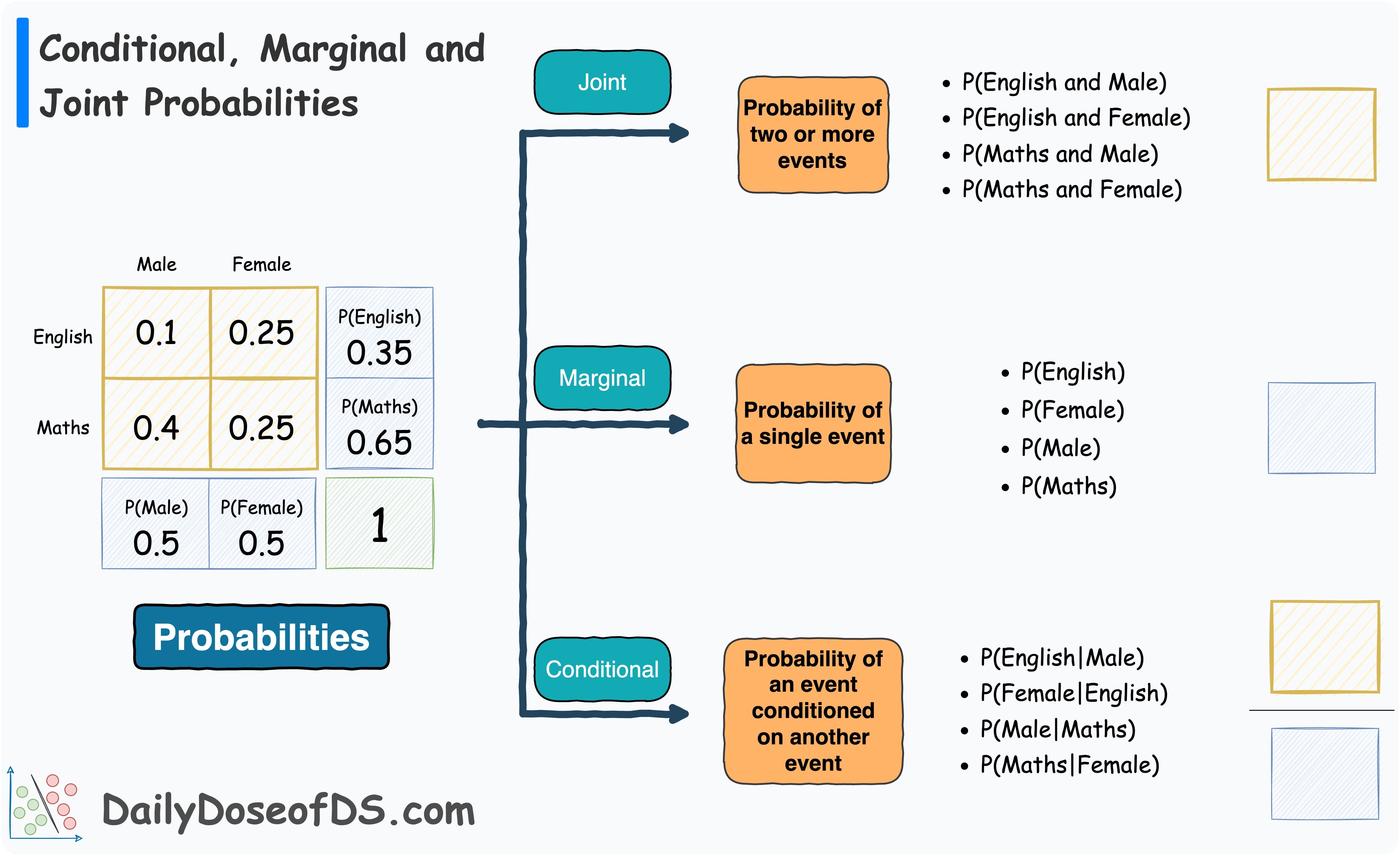
The image below provides a final, compact visual summary of the three probability types and their notation.
Practice and Application
Now it's your turn to apply these concepts. The following image presents a practical problem involving data from a survey in Yellowstone National Park.
Your task:
- Read the problem description and study the contingency table.
- Try to answer the three questions posed at the bottom of the image on your own. For each question, identify which type of distribution is being asked for, calculate the required percentages, and write down a one-sentence interpretation.
- Once you are done, compare your work with the answers provided in the image.
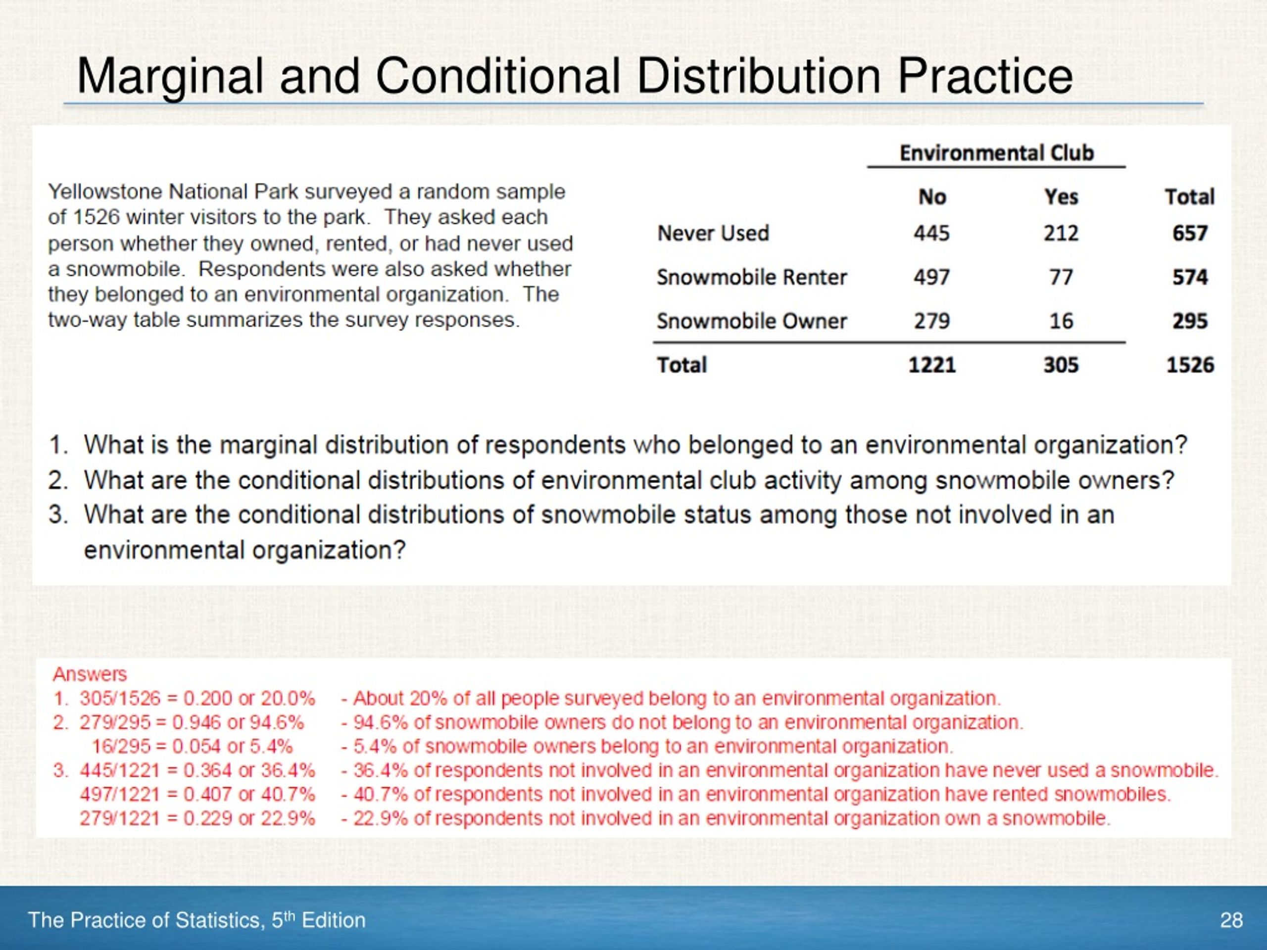
Let's briefly review the logic for the practice problem:
- Question 1 asks for the "distribution of opinion about snowmobile use." This is asking for the marginal distribution of the snowmobile variable, as it doesn't mention environmental club membership. You find this by dividing each row total by the grand total ().
- Question 2 asks for the distribution of opinion among members of an environmental club. The phrase "among" is a clear signal for a conditional distribution. You must restrict your focus to the 119 people in the "Yes" column and calculate percentages using 119 as your denominator.
- Question 3 also asks for a conditional distribution, but this time the condition is being a "Never Used" respondent. You restrict your analysis to the top row and use the row total of 495 as your denominator to find the percentage of that group who are or are not club members.
By comparing the conditional distribution from question 2 to the marginal distribution from question 1, you can see a clear relationship. Environmental club members are far more likely to have never used a snowmobile (62%) compared to the general visitor population (38%).
Conclusion
In this lesson, we focused on the mechanics of extracting meaning from a contingency table by calculating and interpreting its underlying distributions.
Key Takeaways:
- Joint Distribution: The probability of two events occurring together. Calculated as
(cell count) / (grand total). - Marginal Distribution: The overall probability distribution for a single variable. Calculated as
(row or column total) / (grand total). - Conditional Distribution: The probability distribution of one variable, restricted to a single category of another. Calculated as
(cell count) / (row or column total). This is the most critical distribution for assessing relationships.
Preview of the Next Lesson:
Comparing conditional distributions visually is a great first step, but it's not a formal statistical measure. In our next lesson, we will quantify the difference between two conditional probabilities by defining, computing, and interpreting our first formal measure of association for a 2x2 table: the difference in proportions.