Difference in Proportions for 2x2 Tables

1. Defining the Difference in Proportions

In the previous lesson, you saw that a relationship might exist if $P(\text{Outcome}|\text{Group A})$ is different from $P(\text{Outcome}|\text{Group B})$. The simplest way to quantify this difference is to subtract one from the other. This is the entire idea behind the difference in proportions.

Let's consider a standard 2x2 contingency table, which compares an exposure (e.g., smoking) to an outcome (e.g., lung cancer).

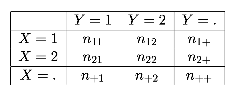
We are interested in comparing the proportion of individuals who experience the outcome (Y=1) in the exposed group (X=1) versus the unexposed group (X=2). These are the two conditional probabilities:

• Proportion in Group 1 (Exposed): ${\pi }_1=P(Y=1|X=1)=\frac{n_{11}}{n_{1+}}$
• Proportion in Group 2 (Unexposed): ${\pi }_2=P(Y=1|X=2)=\frac{n_{21}}{n_{2+}}$

The Difference in Proportions (DP) is simply the difference between these two values:

You will encounter several names for this same concept, all of which are used interchangeably:

• Risk Difference (RD)
• Attributable Risk (AR)
• Absolute Risk Reduction (ARR) (if the difference represents a decrease in risk)

To see this concept explained, the following video provides a concise and clear overview.

The video you just watched framed the difference in proportions as an additive change. Another powerful way to interpret this value is as the "excess risk"—the additional risk that comes from the exposure.

Let's watch one more short clip to solidify this interpretation.

2. Computing the Difference in Proportions

Now that we have a solid conceptual understanding, let's walk through a concrete calculation. The image below shows data from a hypothetical study on the relationship between heavy drinking and lung cancer.

Let's break down the calculation shown in the image:

1. Identify the Groups and Outcome:

   • Group 1 (Exposed): Heavy Drinkers
   • Group 2 (Unexposed): Non-Drinkers
   • Outcome: Lung Cancer (Yes)

2. Calculate the Proportion (Risk) for Each Group:

   • Risk for Heavy Drinkers ($p_1$): There are 100 heavy drinkers, and 30 got lung cancer. The risk is $\frac{30}{100}=0.30$.
   • Risk for Non-Drinkers ($p_2$): There are 100 non-drinkers, and 10 got lung cancer. The risk is $\frac{10}{100}=0.10$.

3. Calculate the Difference in Proportions (Risk Difference):

   • $RD=p_1-p_2=0.30-0.10=0.20$.

Interpretation: The risk of developing lung cancer is 0.20, or 20 percentage points, higher for heavy drinkers compared to non-drinkers in this sample. This 20% is the "excess risk" attributable to heavy drinking.

The image also shows the calculation of a 95% confidence interval: (0.09, 0.31). This interval gives us a range of plausible values for the true risk difference in the entire population. Since the interval does not contain 0, we can be reasonably confident that there is a real difference in risk between the two groups. We will explore confidence intervals and hypothesis testing in more detail later.

3. Why the Difference in Proportions is Important

You might ask: why not just use a ratio? As you'll see in the next lesson, we can. However, the difference in proportions, or absolute risk difference, has a unique and crucial role in interpretation, especially for understanding the practical, real-world impact of a finding.

The following reading explains this very clearly.

The key takeaway from the reading is that context matters. A relative measure can make a small effect seem dramatic. The difference in proportions grounds our analysis in reality.

Consider this example:

• Scenario A: A new teaching method reduces the failure rate on an exam from 4% to 2%.
• Scenario B: A new public health policy reduces the incidence of a common disease from 40% to 20%.

In both scenarios, the risk is halved (a 50% relative reduction). However, the absolute impact is vastly different:

• In Scenario A, the difference in proportions is $0.04-0.02=0.02$. The policy prevents 2 failures for every 100 students.
• In Scenario B, the difference in proportions is $0.40-0.20=0.20$. The policy prevents 20 cases of disease for every 100 people.

The difference in proportions makes the enormous difference in public health significance immediately obvious, whereas focusing only on the "50% reduction" would be misleading. This is a core part of the "functional understanding" you're aiming for: knowing which statistic tells the most relevant story.

Conclusion

In this lesson, we introduced our first formal measure of association for a 2x2 table. You learned how to define, compute, and, most importantly, interpret the difference in proportions.

Key Takeaways:

• The difference in proportions (also called risk difference or attributable risk) is calculated by subtracting the conditional proportion of an outcome in one group from that in another group (${\pi }_1-{\pi }_2$).
• It measures the absolute difference in risk and is interpreted in percentage points (e.g., "a 5 percentage point increase in risk").
• This measure represents the excess risk attributable to the exposure.
• It is crucial for evaluating the practical significance or real-world impact of an exposure or intervention, as it is not inflated by low baseline risks.

Preview of the Next Lesson:

While subtracting proportions gives us a measure of absolute difference, dividing them gives a measure of relative difference. In our next lesson, we will explore this second fundamental measure of association: the relative risk.