Beyond OLS: Handling Non-Normal Responses

1. The Core Assumptions of Ordinary Linear Regression

As you know from your background in basic regression, OLR is a powerful tool, but its validity rests on several key assumptions about the data. The most important ones for our discussion are:

1. Normality of Residuals: The errors, or the differences between the observed and predicted values ($Y-\hat{Y}$), are assumed to be normally distributed with a mean of zero.
2. Homoscedasticity (Constant Variance): The variance of the residuals is assumed to be constant across all levels of the predictor variable(s).
3. Linearity: The relationship between the outcome variable and the predictor variable(s) is assumed to be linear.

When our outcome variable isn't a continuous, normally distributed measure, these assumptions often break down dramatically. Let's see how.

2. The Problem with Binary Outcomes

Imagine you want to model a binary outcome, like whether a patient survives (1) or does not survive (0), based on a continuous predictor like age. Let's explore why forcing a straight line through this data is problematic.

The following reading details the conceptual and statistical issues that arise.

As the reading explains, there are two fundamental flaws:

A. The Conceptual Problem: Nonsensical Predictions

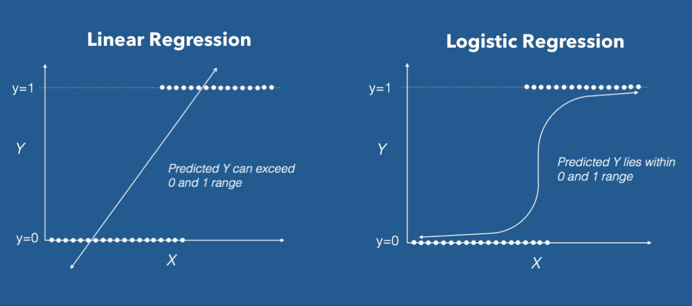
A binary outcome, when thought of as a probability, must be between 0 and 1. However, a linear regression model is unbounded; its prediction line extends infinitely in both directions. This means for low or high values of the predictor, the model can predict probabilities less than 0 or greater than 1, which are logically impossible.

The image below illustrates this perfectly. The straight line (linear regression) ventures below 0 and above 1, while the S-shaped curve (logistic regression, a type of GLM) correctly constrains the predictions within this valid range.

B. The Statistical Problem: Violated Assumptions

1. Non-Normal Residuals: For any given predictor value, the outcome can only be 0 or 1. This means the residuals (the errors) can only take on two possible values. A distribution with only two points is fundamentally not a normal distribution, violating a core assumption of OLR.
2. Heteroscedasticity (Non-Constant Variance): The variance of a binary outcome depends on its mean (the probability, $p$). The variance is given by $p(1-p)$. It is largest when $p=0.5$ and smallest when $p$ is near 0 or 1. Since the probability $p$ changes as our predictor variable changes, the variance of the residuals also changes. This violates the assumption of homoscedasticity.

3. The Problem with Count Data

Now let's consider another common data type: counts. Examples include the number of emails received per hour, the number of defects in a batch of products, or the number of patient visits in a year. Using OLR here is just as problematic.

This short video provides a clear explanation.

To summarize the video and expand on the points:

1. Discrete Nature: Count data consists of non-negative integers (0, 1, 2, ...). OLR assumes a continuous outcome, which is a mismatch.
2. Nonsensical Predictions: Just as with binary data, the linear model is unbounded and can predict negative counts (e.g., -0.7 patient visits), which are meaningless.
3. Skewed Distribution: Count data, especially for rare events, is often highly skewed to the right. There's a pile-up of observations at zero and a long tail of larger values. This is not the symmetric, bell-shaped normal distribution that OLR assumes.
4. Mean-Variance Relationship: For many types of count data (like those following a Poisson distribution), the variance is equal to the mean. As the average count increases, the variability around that average also increases. This directly violates the OLR assumption of homoscedasticity (constant variance).

4. What Are the Practical Consequences?

You might ask, "So what if some assumptions are violated? Does it really matter in practice?" The answer is a resounding yes. Using a model whose assumptions don't match the data's underlying structure leads to invalid statistical inference.

The following video segment explains this critical point.

As the video highlights, when you use OLR on data that is clearly not normal (like binary or count data), you are using the wrong probability distribution to calculate your statistics. The practical consequences are severe:

• Incorrect p-values: You are more likely to make a Type I error—incorrectly concluding that there is a significant effect when there isn't one.
• Inaccurate Confidence Intervals: The confidence intervals around your coefficient estimates will be wrong, giving you a false sense of precision about your findings.

In short, your model's conclusions cannot be trusted.

Conclusion

In this lesson, we established the fundamental motivation for moving beyond Ordinary Linear Regression. We've seen that for both binary and count outcomes, OLR fails on both conceptual and statistical grounds.

Key Takeaways:

• OLR is unsuitable for binary outcomes because it can produce nonsensical predictions outside the 0-1 range, and the data violates the assumptions of normal residuals and constant variance (homoscedasticity).
• OLR is unsuitable for count data because it can predict impossible negative counts, and count data is typically discrete, skewed, and exhibits non-constant variance.
• Violating these core assumptions leads to unreliable statistical inference, including inaccurate p-values and confidence intervals.

These failures are not just minor technicalities; they are fundamental flaws that necessitate a more appropriate tool. This tool is the Generalized Linear Model.

Preview of the Next Lesson:

Now that we know why we need a new approach, our next lesson will introduce the elegant solution provided by GLMs. We will break down the three core components of every GLM—the Random Component, the Systematic Component, and the Link Function—and see how they work together to correctly model the very types of data that cause OLR to fail.