CMH Test for Stratified 2x2 Tables

1. Homogeneity vs. Heterogeneity (Effect Modification)

When we stratify an analysis, one of two things can be true:

1. Homogeneous Association: The strength of the association between the exposure and outcome is essentially the same in every stratum. The stratum-specific odds ratios are all estimating the same underlying value. In this case, calculating a single common odds ratio is a valid and useful way to summarize the overall effect.

2. Heterogeneity of Association (or Effect Modification): The strength, or even the direction, of the association is different across the strata. The stratifying variable is said to modify the effect of the exposure on the outcome.

Imagine testing a new drug.

• Homogeneity: The drug reduces the odds of an adverse event by 30% in both younger and older patients. The effect is consistent.
• Heterogeneity/Effect Modification: The drug reduces the odds of an adverse event by 60% in younger patients but increases the odds by 10% in older patients. The effect is not consistent; age modifies the drug's effect.

In the case of heterogeneity, calculating a single "average" effect would be deeply misleading. It might suggest the drug has a small positive effect overall, completely hiding the fact that it is harmful to a specific subgroup. When effect modification is present, you must report and interpret the stratum-specific odds ratios individually.

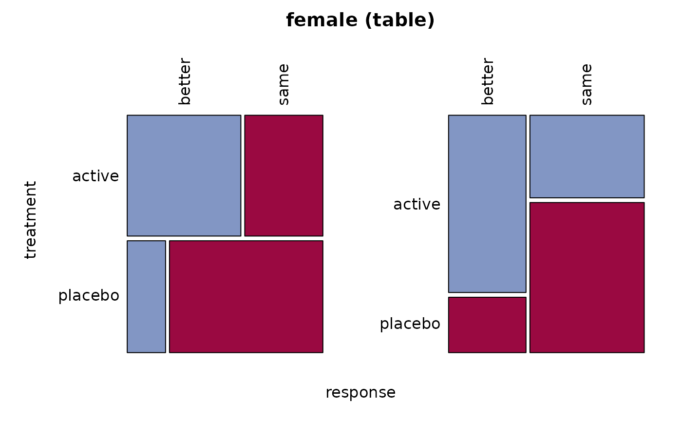
The two mosaic plots below give a visual sense of heterogeneity. They show the association between treatment and response for females, but in two different (hypothetical) studies or strata. Notice how the pattern of association is visibly different between the left and right plots.

2. Testing for Homogeneity: The Breslow-Day Test

To move beyond visual inspection, we use a formal hypothesis test to check for homogeneity. The most common one is the Breslow-Day test.

• Null Hypothesis ($H_0$): The odds ratios are homogeneous across all strata. (${\theta }_1={\theta }_2=\cdots ={\theta }_k$)
• Alternative Hypothesis ($H_1$): The odds ratios are not all equal (at least one is different).

Interpreting the Result:

• A high p-value (e.g., > 0.05) suggests there is no statistical evidence to reject the null hypothesis of homogeneity. We can proceed with the CMH test and report the common odds ratio.
• A low p-value (e.g., ≤ 0.05) provides evidence against homogeneity. We conclude that effect modification is present. We should stop and report the individual odds ratios for each stratum instead of a single common odds ratio.

Let's read a formal description of this assumption and the test.

3. A Complete Workflow for Stratified Analysis

With the Breslow-Day test, we can now define a complete workflow for analyzing stratified 2x2 tables.

1. Stratify the data into separate 2x2 tables, one for each level of the confounding variable.
2. Examine the stratum-specific odds ratios to get a preliminary feel for their consistency.
3. Perform the Breslow-Day test for homogeneity.
   • If the p-value is large: The homogeneity assumption holds. Proceed to steps 4 and 5.
   • If the p-value is small: Stop. There is effect modification. Report the individual stratum-specific odds ratios and conclude that the association differs across levels of the stratifying variable. Do not proceed.
4. Perform the Cochran-Mantel-Haenszel (CMH) test. This tests the null hypothesis that the common odds ratio equals 1 (i.e., no association).
5. Calculate and report the Mantel-Haenszel common odds ratio and its confidence interval. This provides the single, adjusted estimate of the association's strength.

Let's see this workflow in action using R, a tool you'll frequently use in data science.

Analysis of the Titanic Data

Let's apply our workflow to the Titanic data from the reading.

1. Stratify: The data is stratified by Class (1st, 2nd, 3rd, Crew).
2. Examine ORs: The stratum-specific odds ratios for female vs. male survival are calculated as:
   • 1st Class: 67.1
   • 2nd Class: 44.1
   • 3rd Class: 4.1
   • Crew: 23.3
     These values vary quite a bit, suggesting that the survival advantage of being female was much stronger in 1st class than in 3rd class. This already hints at heterogeneity.
3. Test for Homogeneity: The BreslowDayTest output shows p-value < 2.2e-16.
   • This p-value is extremely small, so we reject the null hypothesis of homogeneity.
   • Conclusion: There is significant effect modification. The association between sex and survival depends on passenger class. Therefore, it is inappropriate to report a single common odds ratio. The correct approach is to report the individual odds ratios we examined in step 2.

4. Interpreting Software Output: The Homogeneous Case

The Titanic example showed us what to do when heterogeneity is present. Now, let's look at an example where the association is homogeneous, using a typical output from statistical software like SAS.

The example below analyzes data from a clinical trial, where the outcome is response to treatment (TRTP), the exposure is SEX, and the data is stratified by age group (AGEGR1).

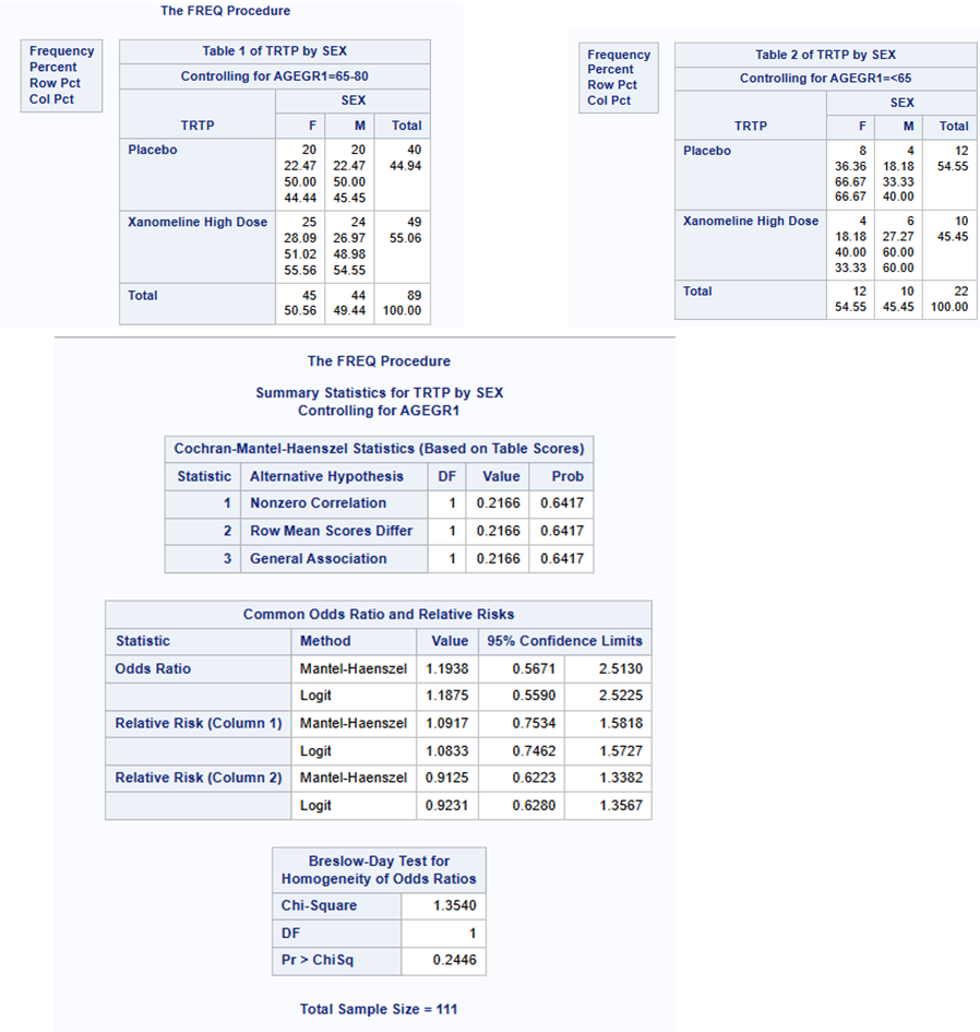
Let's walk through this output using our workflow.

1. Stratify: The output shows "Table 1" for age group 65-80 and "Table 2" for age group <65.
2. Examine ORs: You would calculate the odds ratio for each table (not shown directly, but would be the first step in a manual analysis).
3. Test for Homogeneity: Look at the Breslow-Day Test for Homogeneity of Odds Ratios.
   • Let's assume the Pr > ChiSq (p-value) is large, for instance, 0.85.
   • Conclusion: We fail to reject the null hypothesis. We can assume the odds ratios are homogeneous across age groups. We proceed.
4. Perform CMH Test: Now, look at the Cochran-Mantel-Haenszel Statistics. The statistic for "General Association" tests if the common odds ratio is 1.
   • Let's assume the Prob (p-value) is 0.03.
   • Conclusion: Since p < 0.05, we reject the null hypothesis of no association. There is a statistically significant association between sex and treatment response, after controlling for age.
5. Report Common Odds Ratio: Finally, look at the Estimates of the Common Odds Ratio.
   • The "Mantel-Haenszel" estimate is, for example, 2.5 with a 95% Confidence Interval of (1.1, 5.7).
   • Final Interpretation: "After controlling for age, the odds of a positive response for one sex were 2.5 times the odds for the other sex (95% CI: 1.1–5.7). This association is statistically significant (p=0.03)."

This structured approach ensures your analysis is both statistically sound and easy to interpret.

Conclusion

This lesson has equipped you with the final, crucial piece of the stratified analysis puzzle: the test for homogeneity. You now have a complete framework for analyzing the relationship between two categorical variables while controlling for a third.

Key Takeaways:

• Effect modification (heterogeneity) occurs when the association between an exposure and outcome differs across strata. When it is present, you must report stratum-specific results.
• The Breslow-Day test is used to formally check the assumption of homogeneous association.
• A full CMH analysis involves a clear workflow: first test for homogeneity, and only if it holds, proceed to interpret the CMH test for association and the common odds ratio.

Preview of the Next Lesson:

We have mastered how to control for a single, categorical confounding variable using stratification. But what happens when you have multiple confounders (age, sex, location)? Or when a confounder is continuous (like blood pressure)? Stratifying data into ever-smaller cells quickly becomes impractical.

This limitation provides the perfect motivation for our next topic. We will move from stratification to model-based approaches, beginning with the foundations of Generalized Linear Models (GLMs). GLMs provide a powerful and flexible framework to handle these more complex scenarios, and they are a cornerstone of modern data science.