Log-Linear Models for Contingency Tables

1. The Core Idea: Modeling Cell Counts

At its heart, a contingency table is a grid of observed counts. A log-linear model provides a systematic way to describe the expected counts in each cell based on the levels of the categorical variables that define the table.

The fundamental idea is surprisingly straightforward. As the name suggests, it is a linear model for the logarithm of the expected cell frequency.

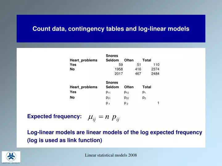
Why use the logarithm? In contingency tables, the relationships between cell probabilities are naturally multiplicative (e.g., under independence, ${\pi }_{ij}={\pi }_{i+}\times {\pi }_{+j}$). Taking the log transforms these multiplicative relationships into a simple, additive linear model. This puts the analysis into the familiar framework of linear models, which you know from regression and ANOVA.

We typically assume the count in each cell, $n_{ijk}$, follows a Poisson distribution with a mean ${\mu }_{ijk}$ equal to that cell's expected count. This provides the direct link from our previous lessons on Poisson regression to the analysis of contingency tables.

2. Building Blocks: Log-Linear Models for Two-Way Tables

To understand how the models represent association, let's start with a simple $I\times J$ two-way table. There are two primary models of interest.

Let's summarize the key ideas from that reading.

The Model of Independence

The log-linear model for independence between two variables, A and B, is:

• $\lambda$ is the overall mean effect (like an intercept).
• ${\lambda }_i^A$ is the main effect for variable A, representing the deviation from the overall mean for being in row $i$.
• ${\lambda }_j^B$ is the main effect for variable B, representing the deviation for being in column $j$.

Critically, there is no interaction term. This model structure asserts that the expected count is determined by an overall level, a row effect, and a column effect, with no special adjustment for being in a specific ($i,j$) cell. This is the log-linear representation of the null hypothesis that variables A and B are independent. In this model, the odds ratio between the variables is always 1.

The Saturated Model

The saturated model allows for association between A and B:

This model adds the crucial interaction term, ${\lambda }_{ij}^{AB}$.

• The ${\lambda }_{ij}^{AB}$ term represents the association between variables A and B. It is a specific adjustment for the combination of row $i$ and column $j$ that cannot be explained by the main effects alone.
• If ${\lambda }_{ij}^{AB}=0$ for all $i$ and $j$, the saturated model simplifies to the independence model.
• The strength of the association (measured by the odds ratio) is directly related to these interaction parameters.

This model is called "saturated" because it has exactly as many parameters as there are cells in the table. Consequently, it will always fit the data perfectly (${\hat{\mu }}_{ij}=n_{ij}$). Its main purpose is to serve as the most complex model, a baseline against which we can compare simpler models like the independence model.

3. Visualizing Association Structure

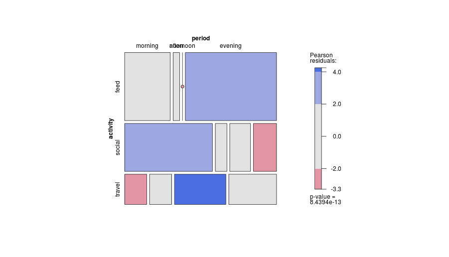
A log-linear model aims to capture the structure of dependencies in a contingency table. A mosaic plot is a graphical tool that helps visualize this same structure.

4. Models for Three-Way Tables: Describing Complex Relationships

The true power of log-linear models emerges when we analyze tables with three or more variables. Here, we can model much more nuanced association structures than simple independence.

The saturated model for three variables (A, B, C) is:

By including or excluding specific interaction terms, we can represent different hypotheses about the relationships among A, B, and C.

Let's review the key association structures you can model, using a common shorthand notation where terms in parentheses represent the highest-order interaction terms in the model.

• Model of Complete Independence: (A, B, C)

  • Structure: $\log ({\mu }_{ijk})=\lambda +{\lambda }_i^A+{\lambda }_j^B+{\lambda }_k^C$
  • Interpretation: This is the simplest model, containing only main effects. It specifies that all three variables are mutually independent of one another. There are no two-way or three-way interactions. This corresponds to the hypothesis that the joint probability is the product of the marginal probabilities: ${\pi }_{ijk}={\pi }_{i..}{\pi }_{.j.}{\pi }_{..k}$.

• Model of Conditional Independence: (AC, BC)

  • Structure: $\log ({\mu }_{ijk})=\lambda +{\lambda }_i^A+{\lambda }_j^B+{\lambda }_k^C+{\lambda }_{ik}^{AC}+{\lambda }_{jk}^{BC}$
  • Interpretation: This model hypothesizes that variables A and B are independent, conditional on the level of C. It includes interaction terms for (A,C) and (B,C) but crucially omits the (A,B) interaction term. For example, this model could represent a situation where exercise (A) and diet (B) are only related through their mutual association with health consciousness (C). Once you account for health consciousness, there is no direct association between exercise and diet.

• Model of Homogeneous Association: (AB, AC, BC)

  • Structure: $\log ({\mu }_{ijk})=\lambda +{\lambda }_i^A+{\lambda }_j^B+{\lambda }_k^C+{\lambda }_{ij}^{AB}+{\lambda }_{ik}^{AC}+{\lambda }_{jk}^{BC}$
  • Interpretation: This is one of the most useful models. It lacks the three-way interaction term (${\lambda }_{ijk}^{ABC}$). It specifies that every pair of variables is associated, but the strength of the association between any two variables is the same at every level of the third variable. For example, the odds ratio describing the association between smoking (A) and lung cancer (B) is constant across all age groups (C). If the three-way interaction term ${\lambda }_{ijk}^{ABC}$ were present and significant, it would mean that this odds ratio changes depending on the age group.

Conclusion

Today, we've unpacked the conceptual foundation of log-linear models. You've seen that they are not just an abstract statistical technique but a descriptive language for articulating and testing specific theories about how categorical variables relate to one another.

Key Takeaways:

• Log-linear models represent the association structure in a contingency table by building a linear model for the log of the expected cell counts.
• The parameters in the model correspond to main effects (overall distribution of variables) and interaction effects (associations between variables).
• For a two-way table, the independence model has no interaction term, while the saturated model includes a two-way interaction term that captures the association.
• For three-way tables, different models can represent complete independence, conditional independence, and homogeneous association by strategically including or excluding various interaction terms.
• The absence of a three-way interaction term ${\lambda }_{ijk}^{ABC}$ implies that the association between any two variables is consistent across all levels of the third.

Preview of the Next Lesson:
We've focused on what log-linear models represent. In our next lesson, we will formalize the connection between Poisson regression and log-linear models. You will see that fitting a log-linear model is practically equivalent to running a Poisson regression on the table's cell counts, which will bridge the theory from today with the practical skills of model fitting and interpretation.