Chi-Square Test and Saturated Log-Linear Models

1. Reframing the Chi-Square Test

Let's start by revisiting the Pearson chi-square test for independence in a two-way table. You'll recall that its purpose is to test the null hypothesis ($H_0$) that the two categorical variables are independent.

The test statistic is calculated as:

The core of this test lies in the comparison between the observed counts in each cell and the expected counts we would see if the null hypothesis of independence were true.

Now, let's look at this through the lens of log-linear models.

• What are the "Expected" counts? The expected counts for the chi-square test are calculated under the assumption of independence. These are precisely the counts predicted by the log-linear model of independence.

  $$\log ({\mu }_{ij})=\lambda +{\lambda }_i^A+{\lambda }_j^B$$

  The fitted values, ${\hat{\mu }}_{ij}$, from this model are identical to the expected counts, $E_{ij}$, used in the standard chi-square test formula.

• What are the "Observed" counts? The observed counts, $n_{ij}$, are the actual data. The log-linear model that perfectly reproduces the observed counts is the saturated model.

  $$\log ({\mu }_{ij})=\lambda +{\lambda }_i^A+{\lambda }_j^B+{\lambda }_{ij}^{AB}$$

  Because this model has a parameter for every cell, its fitted values are the observed counts themselves: ${\hat{\mu }}_{ij}=n_{ij}$.

Therefore, the chi-square test is fundamentally a goodness-of-fit test. It measures how well the simpler independence model fits the data, using the saturated model (i.e., the observed data) as the benchmark for a perfect fit.

The following reading makes this connection explicit.

2. A Formal Model Comparison: The Likelihood Ratio Test

The Pearson chi-square statistic ($X^2$) is one way to measure the distance between the observed and expected counts. Another, which is more directly tied to the logic of model comparison, is the Likelihood Ratio Test statistic, often denoted as $G^2$.

For contingency tables, the $G^2$ statistic is calculated as:

Just like the Pearson $X^2$, $G^2$ follows a chi-square distribution under the null hypothesis and is used to test for independence. In practice, $X^2$ and $G^2$ usually give very similar results.

The power of the $G^2$ statistic is that it provides a general way to compare nested models. A simpler model (e.g., independence) is "nested" within a more complex model (e.g., saturated) if it can be obtained by setting some parameters of the complex model to zero.

The chi-square test of independence can be formally stated as a likelihood ratio test comparing two models:

• Null Model ($M_0$): The log-linear model of independence.
• Alternative Model ($M_1$): The saturated log-linear model.

The test statistic is the difference in their deviances (a measure of model fit, where lower is better). The deviance of the saturated model is always 0 because it fits perfectly. Therefore, the $G^2$ for the test of independence is simply the deviance of the independence model.

In essence, the chi-square test of independence asks: "Is the fit of the independence model significantly worse than a perfect fit?"

3. Seeing the Connection in Practice

This idea that common statistical tests are just specific versions of linear (or generalized linear) models is a powerful concept in modern statistics. It unifies many different procedures under a single framework.

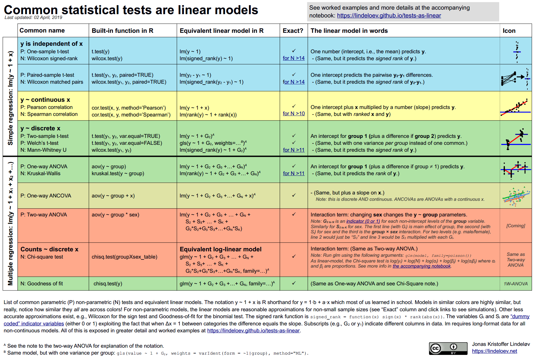
Let's look at how this plays out with code. We can perform a chi-square test of independence in two ways: using the standard chisq.test() function or by fitting and comparing two log-linear models. The results will be the same.

As you saw in the reading, the analysis produces a p-value for the mood:sex interaction term in the log-linear model. This p-value is identical to the one produced by the standard chisq.test.

This confirms our key insight: testing for independence is equivalent to testing whether the interaction term (${\lambda }_{ij}^{AB}$) in the saturated log-linear model is zero.

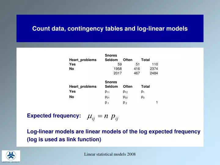
Conclusion

Today we connected the dots between two important concepts: the familiar chi-square test and the more general framework of log-linear models. This new perspective is more than a theoretical curiosity; it's a gateway to more advanced analyses. While the chi-square test tells you if there's an association, analyzing different log-linear models allows you to describe how variables are associated, especially in complex, multi-way tables.

Key Takeaways:

• The chi-square test for independence compares observed cell counts to the expected cell counts calculated under the assumption of independence.
• The saturated log-linear model perfectly reproduces the observed cell counts.
• The log-linear model of independence perfectly reproduces the expected cell counts used in the chi-square test.
• Therefore, the chi-square test of independence is implicitly a goodness-of-fit test that compares the fit of the independence model against the saturated model.
• Testing for independence is equivalent to testing the null hypothesis that the interaction term in the saturated log-linear model is zero.

Preview of the Next Lesson:
We've now established what log-linear models are and how they relate to classical tests. In the next lesson, we will solidify the connection between Poisson regression and log-linear models. You'll learn that fitting a log-linear model is practically accomplished by running a Poisson regression, which provides the computational engine for everything we've discussed.